Comparing two columns in Excel to identify matches or differences can be efficiently achieved using the VLOOKUP function, and COMPARE.EDU.VN is here to guide you through the process. This method allows you to find common values or spot missing data between two lists, enhancing your data analysis capabilities. Learn how to leverage VLOOKUP along with functions like IFNA, FILTER, and XLOOKUP to streamline your spreadsheet tasks, making data comparison and analysis easier and more accurate.
1. What is VLOOKUP and How Can It Help Compare Two Columns in Excel?
VLOOKUP, or Vertical Lookup, is an Excel function that searches for a specific value in the first column of a range and returns a value from any cell on the same row of that range. This function is particularly useful when you need to compare two columns to find matches or identify differences. By using VLOOKUP, you can quickly determine if data points from one list exist in another, thereby facilitating data analysis and decision-making.
To effectively use VLOOKUP, you need to understand its syntax:
VLOOKUP(lookup_value, table_array, col_index_num, [range_lookup])
- lookup_value: The value you want to search for in the first column of the table array.
- table_array: The range of cells where VLOOKUP will search for the lookup_value.
- col_index_num: The column number within the table_array from which the matching value will be returned.
- range_lookup: A logical value (TRUE or FALSE) that specifies whether you want an approximate or exact match. Use FALSE for an exact match, which is common when comparing columns.
For example, if you have a list of customer IDs in column A and another list in column B, you can use VLOOKUP to check if each ID in column A exists in column B. This way, you can identify which customers are present in both lists or which are unique to each list.
2. How Can You Use a Basic VLOOKUP Formula to Compare Two Columns?
A basic VLOOKUP formula can effectively compare two columns by searching for values from one column in another. Here’s how to set it up:
-
Identify the Columns: Determine which column contains the values you want to look up (List 1) and which column you want to search within (List 2).
-
Enter the Formula: In a new column next to List 1, enter the VLOOKUP formula.
=VLOOKUP(A2, $C$2:$C$9, 1, FALSE)A2is the first value in List 1 that you want to find in List 2.$C$2:$C$9is the range of cells containing List 2. The dollar signs make this an absolute reference, which prevents the range from changing when you copy the formula down.1indicates that you want to return the value from the first column of List 2 if a match is found.FALSEensures that VLOOKUP looks for an exact match.
-
Apply the Formula: Drag the formula down to apply it to all the values in List 1.
-
Interpret the Results: If VLOOKUP finds a match, it will return the matching value from List 2. If it doesn’t find a match, it will return a
#N/Aerror.
This basic formula provides a straightforward way to compare two columns and identify common values. However, to enhance the usability and clarity of the results, you might want to handle the #N/A errors, as discussed in the next section.
3. How Do You Disguise #N/A Errors When Using VLOOKUP?
The #N/A errors returned by VLOOKUP when no match is found can be confusing. To make your spreadsheet more user-friendly, you can disguise these errors using the IFNA or IFERROR functions.
-
Using the IFNA Function: The
IFNAfunction allows you to replace#N/Aerrors with a value of your choice, such as a blank cell or custom text.=IFNA(VLOOKUP(A2, $C$2:$C$9, 1, FALSE), "")This formula returns an empty string (
"") instead of#N/A, resulting in a blank cell. -
Using the IFERROR Function: The
IFERRORfunction is similar toIFNAbut catches all types of errors, not just#N/A.=IFERROR(VLOOKUP(A2, $C$2:$C$9, 1, FALSE), "Not in List 2")This formula returns the text “Not in List 2” when VLOOKUP results in any error.
-
Custom Text: You can also use custom text to provide more context. For example:
=IFNA(VLOOKUP(A2, $C$2:$C$9, 1, FALSE), "Not Found")This will display “Not Found” if a value from List 1 is not found in List 2.
By disguising #N/A errors, you create a cleaner, more informative spreadsheet that is easier to interpret, especially for users who may not be familiar with Excel error codes.
4. How Can You Compare Two Columns in Different Excel Sheets Using VLOOKUP?
When the columns you need to compare are located on different sheets within the same Excel workbook, you can still use VLOOKUP with a slight modification to the formula. Here’s how:
-
Reference the Sheet: When specifying the table_array argument, include the sheet name followed by an exclamation mark (
!) before the cell range.=IFNA(VLOOKUP(A2, Sheet2!$A$2:$A$9, 1, FALSE), "")In this formula,
Sheet2!$A$2:$A$9refers to the range A2 to A9 on Sheet2. -
Select the Range: You can also start typing the formula in your main sheet, then switch to the other sheet and select the range using the mouse. Excel will automatically add the appropriate sheet reference to the formula.
-
Apply the Formula: Drag the formula down to apply it to all the values in List 1 on the first sheet.
This approach allows you to compare data across different sheets, making it easier to consolidate and analyze information from multiple sources within the same workbook.
5. How Do You Compare Two Columns and Return Common Values (Matches)?
To extract a list of common values between two columns, you can use VLOOKUP in combination with filtering techniques or dynamic array functions.
-
Using Auto-Filter: After applying the VLOOKUP formula (with error handling), you can use Excel’s auto-filter to display only the common values.
- Apply the VLOOKUP formula with
IFNAorIFERRORto handle errors. - Select the column with the VLOOKUP results.
- Go to the “Data” tab and click on “Filter”.
- Click the filter arrow in the column header and uncheck the “Blanks” option.
This will display only the rows where VLOOKUP found a match, effectively showing the common values between the two columns.
- Apply the VLOOKUP formula with
-
Using the FILTER Function: In Excel 365 and Excel 2021, you can use the
FILTERfunction to dynamically return a list of common values.=FILTER(A2:A14, IFNA(VLOOKUP(A2:A14, C2:C9, 1, FALSE), "")<>"")A2:A14is the range containing List 1.C2:C9is the range containing List 2.- The
IFNA(VLOOKUP(...), "")<>""part checks for non-blank results from VLOOKUP, indicating a match.
-
Using the ISNA Function: Alternatively, you can use the
ISNAfunction to check for#N/Aerrors and filter accordingly.=FILTER(A2:A14, ISNA(VLOOKUP(A2:A14, C2:C9, 1, FALSE))=FALSE)This formula filters out the values for which VLOOKUP returns an error, displaying only the common values.
-
Using the XLOOKUP Function: The
XLOOKUPfunction, available in Excel 365 and Excel 2021, can simplify the formula even further.=FILTER(A2:A14, XLOOKUP(A2:A14, C2:C9, C2:C9,"")<>"")Because
XLOOKUPcan handle#N/Aerrors internally with the if_not_found argument, the formula is more concise.
By using these methods, you can easily extract and display a list of common values, providing a clear overview of the data points shared between the two columns.
6. How Can You Compare Two Columns and Find Missing Values (Differences)?
To identify the values that are present in one column but missing from another, you can use VLOOKUP in combination with the IF and ISNA functions or the FILTER function.
-
Using IF and ISNA: This method uses a combination of functions to check for missing values.
=IF(ISNA(VLOOKUP(A2, $C$2:$C$9, 1, FALSE)), A2, "")ISNA(VLOOKUP(A2, $C$2:$C$9, 1, FALSE))checks if VLOOKUP returns an#N/Aerror, indicating that the value from List 1 is not found in List 2.- If the value is not found, the formula returns the value from List 1 (
A2). Otherwise, it returns an empty string ("").
-
Using the FILTER Function: In Excel 365 and Excel 2021, you can use the
FILTERfunction to dynamically return a list of missing values.=FILTER(A2:A14, ISNA(VLOOKUP(A2:A14, C2:C9, 1, FALSE)))This formula filters List 1 (
A2:A14) to include only the values for which VLOOKUP returns an#N/Aerror, effectively displaying the missing values. -
Using XLOOKUP for Criteria: You can also use
XLOOKUPto achieve the same result.=FILTER(A2:A14, XLOOKUP(A2:A14, C2:C9, C2:C9,"")="")This formula filters List 1 based on whether
XLOOKUPreturns an empty string for each value, indicating that the value is missing from List 2.
By using these methods, you can easily identify and list the values that are unique to one column, providing valuable insights into the differences between the two datasets.
7. How Do You Use a VLOOKUP Formula to Identify Matches and Differences Between Two Columns?
To identify both matches and differences between two columns and label them accordingly, you can use VLOOKUP in combination with the IF and ISNA/ISERROR functions.
-
Using IF and ISNA: This method adds text labels to indicate whether a value is present in both lists or only in one.
=IF(ISNA(VLOOKUP(A2, $D$2:$D$9, 1, FALSE)), "Not qualified", "Qualified")ISNA(VLOOKUP(A2, $D$2:$D$9, 1, FALSE))checks if VLOOKUP returns an#N/Aerror.- If the value is not found, the formula returns “Not qualified”. If the value is found, it returns “Qualified”.
-
Using the MATCH Function: Another way to achieve the same result is by using the
MATCHfunction.=IF(ISNA(MATCH(A2, $D$2:$D$9, 0)), "Not in List 2", "In List 2")MATCH(A2, $D$2:$D$9, 0)searches for the valueA2in the range$D$2:$D$9. If a match is found, it returns the position of the match; otherwise, it returns an#N/Aerror.ISNAthen checks for the#N/Aerror and returns the appropriate label.
By using these formulas, you can quickly label each value in your list, making it easy to see which values are common to both columns and which are unique to one.
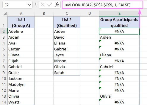
8. How Can You Compare Two Columns and Return a Value From a Third Column?
When you need to compare two columns and return a corresponding value from a third column, VLOOKUP is ideally suited for this task. This is a common scenario when working with tables containing related data.
-
Basic VLOOKUP: Use VLOOKUP to find a match in one column and return a value from another column in the same row.
=VLOOKUP(A3, $D$3:$E$10, 2, FALSE)A3is the value you want to look up.$D$3:$E$10is the range containing the lookup column (D) and the column from which you want to return a value (E).2indicates that you want to return the value from the second column in the range (column E).
-
Handling Errors: Use
IFNAto handle#N/Aerrors and return a custom value or blank cell.=IFNA(VLOOKUP(A3, $D$3:$E$10, 2, FALSE), "") -
Using INDEX and MATCH: For more flexibility, you can use the
INDEXandMATCHfunctions together.=IFNA(INDEX($E$3:$E$10, MATCH(A3, $D$3:$D$10, 0)), "")INDEX($E$3:$E$10)specifies the column from which you want to return a value.MATCH(A3, $D$3:$D$10, 0)finds the row number whereA3is found in the range$D$3:$D$10.
-
Using XLOOKUP: The
XLOOKUPfunction provides a more modern and flexible alternative to VLOOKUP.=XLOOKUP(A3, $D$3:$D$10, $E$3:$E$10, "")A3is the lookup value.$D$3:$D$10is the lookup array.$E$3:$E$10is the return array.""is the value to return if no match is found.
-
Filtering Results: To display only the rows with matching values, you can use the
FILTERfunction.=FILTER(A3:B15, B3:B15<>"")
By combining these techniques, you can efficiently compare two columns and retrieve relevant data from a third column, enhancing your ability to analyze and manipulate data in Excel.
9. What Are Some Alternative Comparison Tools Available for Excel?
While VLOOKUP is a powerful tool for comparing columns in Excel, several alternative tools and functions can offer more specialized or efficient solutions.
- Conditional Formatting: Use conditional formatting to highlight duplicate or unique values in two columns.
- COUNTIF Function: The
COUNTIFfunction can count the number of times a value from one column appears in another, helping you identify matches. - Advanced Filter: Use Excel’s advanced filter to extract unique or common values between two columns.
- Power Query: Power Query (Get & Transform Data) allows you to merge and compare data from multiple sources, including different sheets or workbooks.
- Third-Party Add-ins: Consider using third-party add-ins like Ablebits Ultimate Suite for Excel, which includes tools specifically designed for comparing tables and sheets.
10. Where Can You Find More Resources and Practice Workbooks for Learning VLOOKUP?
To further enhance your skills with VLOOKUP and data comparison in Excel, several resources and practice workbooks are available.
- Microsoft Office Support: The official Microsoft Office support website provides detailed documentation and tutorials on VLOOKUP and other Excel functions.
- Online Courses: Platforms like Coursera, Udemy, and LinkedIn Learning offer courses on Excel, including in-depth modules on VLOOKUP and data analysis.
- Excel Blogs and Forums: Websites like Exceljet, Chandoo.org, and MrExcel offer tips, tricks, and tutorials on using VLOOKUP and other Excel functions.
- YouTube Tutorials: Many Excel experts offer free video tutorials on YouTube, demonstrating how to use VLOOKUP for various data comparison tasks.
By exploring these resources and practicing with sample workbooks, you can gain a deeper understanding of VLOOKUP and improve your ability to compare and analyze data in Excel.
Do you find yourself struggling to compare data and make informed decisions? Visit COMPARE.EDU.VN today! We provide comprehensive and objective comparisons of various products, services, and ideas, tailored to your needs. Whether you’re a student, professional, or consumer, our detailed analyses will help you navigate the complexities of choices and make the best decision.
Address: 333 Comparison Plaza, Choice City, CA 90210, United States
WhatsApp: +1 (626) 555-9090
Website: compare.edu.vn