How To Compare Using Vlookup In Excel is a skill that can greatly enhance your data analysis capabilities. At COMPARE.EDU.VN, we empower you with the knowledge to master this function and efficiently identify matches and differences between datasets. Learn to compare data lists with ease and speed.
Table of Contents
- Understanding the Basics of VLOOKUP for Comparison
- Step-by-Step Guide: Comparing Two Columns Using VLOOKUP
- Advanced Techniques: Handling Errors and Customizing Output
- Comparing Columns Across Different Excel Sheets
- Extracting Common Values (Matches) from Two Columns
- Identifying Missing Values (Differences) Between Two Columns
- Combining VLOOKUP with IF and ISNA for Enhanced Comparison
- Leveraging VLOOKUP to Retrieve Values from a Third Column
- Alternative Methods: INDEX MATCH and XLOOKUP for Comparison
- Streamlining Comparison with Specialized Tools
- Frequently Asked Questions (FAQs) About VLOOKUP Comparison
- Conclusion: Mastering Data Comparison with VLOOKUP and COMPARE.EDU.VN
1. Understanding the Basics of VLOOKUP for Comparison
VLOOKUP (Vertical Lookup) is a powerful Excel function designed to search for a specific value in the first column of a table and then return a value from the same row in a column you specify. When it comes to data comparison, VLOOKUP can be invaluable for identifying matches and differences between two lists or datasets. It searches vertically through a column. VLOOKUP is a fundamental tool for data validation.
The primary purpose of VLOOKUP is to:
- Verify if a value from one list exists in another.
- Extract corresponding data associated with a matched value.
By mastering VLOOKUP, users can significantly streamline their data comparison processes, enabling them to make informed decisions based on accurate and readily available insights.
2. Step-by-Step Guide: Comparing Two Columns Using VLOOKUP
The core principle of using VLOOKUP for comparing two columns involves searching for values from one column (the lookup column) within another column (the table array). Here’s a detailed, step-by-step approach:
2.1 Setting Up Your Data:
- Ensure that your data is organized into two distinct columns in an Excel sheet.
- For this example, let’s consider two columns: “Product IDs” in Column A (List 1) and “Registered Product IDs” in Column B (List 2).
2.2 Writing the VLOOKUP Formula:
In an empty column (e.g., Column C), write the VLOOKUP formula:
=VLOOKUP(A2, $B$2:$B$100, 1, FALSE)
- A2: The lookup value – the first Product ID from List 1.
- $B$2:$B$100: The table array – the range of cells containing List 2 (the registered product IDs). The dollar signs ($) create absolute references, ensuring the range doesn’t change when the formula is dragged down. Adjust this range to match your actual data.
- 1: The column index number – since we’re only interested in knowing whether the value exists in List 2, we specify 1, indicating the first (and only) column in our table array.
- FALSE: Specifies an exact match. VLOOKUP will only return a value if it finds an exact match for the lookup value in the table array.
2.3 Applying the Formula:
Drag the formula down from cell C2 to apply it to all the Product IDs in List 1.
2.4 Interpreting the Results:
- If a Product ID from List 1 is found in List 2, the formula will return that Product ID in Column C.
- If a Product ID from List 1 is not found in List 2, the formula will return a “#N/A” error.
2.5 Refining Results with Conditional Formatting (Optional):
To visually highlight the matches or differences:
- Select Column C (the column with the VLOOKUP formulas).
- Go to “Conditional Formatting” in the “Home” tab.
- Choose “Highlight Cells Rules” and then “Equal To”.
- Enter “#N/A” and choose a formatting style to highlight the cells containing errors (indicating missing values).
- Repeat the process, but this time, choose “Not Equal To” and enter “#N/A” to highlight the cells with matching values.
3. Advanced Techniques: Handling Errors and Customizing Output
While the basic VLOOKUP formula effectively identifies matches and differences, the “#N/A” errors can be visually distracting. Here’s how to handle these errors and customize the output:
3.1 Using IFNA Function:
The IFNA function replaces “#N/A” errors with a specified value. The syntax is:
=IFNA(value, value_if_na)
Modify the original VLOOKUP formula as follows:
=IFNA(VLOOKUP(A2, $B$2:$B$100, 1, FALSE), "Not Found")
This formula will now return “Not Found” instead of “#N/A” for missing values.
3.2 Using IFERROR Function:
The IFERROR function is similar to IFNA but handles all types of errors, not just “#N/A”. The syntax is:
=IFERROR(value, value_if_error)
Modify the original VLOOKUP formula as follows:
=IFERROR(VLOOKUP(A2, $B$2:$B$100, 1, FALSE), "Not Found")
3.3 Customizing Output Based on Match Status:
To display different messages based on whether a match is found, combine VLOOKUP with the IF function:
=IF(ISNA(VLOOKUP(A2, $B$2:$B$100, 1, FALSE)), "Not in List 2", "In List 2")
This formula checks if the VLOOKUP returns an error using the ISNA function. If an error is returned (ISNA is TRUE), it displays “Not in List 2”; otherwise, it displays “In List 2”.
4. Comparing Columns Across Different Excel Sheets
Often, the columns you need to compare reside in different Excel sheets. To accomplish this, you’ll need to use external references in your VLOOKUP formula.
4.1 Referencing Data from Another Sheet:
Assuming List 1 is in Column A of “Sheet1” and List 2 is in Column A of “Sheet2”, the formula in “Sheet1” would be:
=IFNA(VLOOKUP(A2, Sheet2!$A$2:$A$100, 1, FALSE), "Not Found")
The Sheet2!$A$2:$A$100 part of the formula references the range A2:A100 in “Sheet2”.
4.2 Referencing Data from Another Workbook:
When the data is in a different workbook, the reference will include the workbook name in square brackets:
=IFNA(VLOOKUP(A2, '[Workbook2.xlsx]Sheet1'!$A$2:$A$100, 1, FALSE), "Not Found")
5. Extracting Common Values (Matches) from Two Columns
To extract a list of common values without gaps, you can use a combination of VLOOKUP and filtering.
5.1 Using AutoFilter:
- Apply the basic VLOOKUP formula (with IFNA or IFERROR for error handling) to compare the two columns.
- Select the column with the VLOOKUP formulas.
- Go to the “Data” tab and click “Filter”.
- Click the filter dropdown in the VLOOKUP column and uncheck the “Not Found” or “#N/A” option (depending on your error handling formula) to display only the matching values.
5.2 Using the FILTER Function (Excel 365 and Excel 2021):
If you have Excel 365 or Excel 2021, you can use the FILTER function for a dynamic solution:
=FILTER(A2:A100, IFNA(VLOOKUP(A2:A100, B2:B100, 1, FALSE), "")<>"")
This formula dynamically filters List 1 (A2:A100) to include only the values that are found in List 2 (B2:B100).
6. Identifying Missing Values (Differences) Between Two Columns
To find the values that exist in one column but not in the other, you can modify the VLOOKUP formula to specifically identify the missing values.
6.1 Using IF and ISNA:
=IF(ISNA(VLOOKUP(A2, $B$2:$B$100, 1, FALSE)), A2, "")
This formula checks if the VLOOKUP returns an error (using ISNA). If an error is returned (meaning the value is not found in List 2), it displays the value from List 1; otherwise, it displays an empty string.
6.2 Using the FILTER Function (Excel 365 and Excel 2021):
=FILTER(A2:A100, ISNA(VLOOKUP(A2:A100, B2:B100, 1, FALSE)))
This formula dynamically filters List 1 (A2:A100) to include only the values that are not found in List 2 (B2:B100).
7. Combining VLOOKUP with IF and ISNA for Enhanced Comparison
By combining VLOOKUP with IF and ISNA, you can create more sophisticated comparison formulas that provide meaningful insights.
7.1 Identifying Matches and Differences with Text Labels:
=IF(ISNA(VLOOKUP(A2, $B$2:$B$100, 1, FALSE)), "Not in List 2", "In List 2")
This formula displays “Not in List 2” if the value from List 1 is not found in List 2, and “In List 2” if it is found. This is particularly useful for generating reports or dashboards where clear labels are needed.
7.2 Using MATCH Function as an Alternative:
The MATCH function can also be used to identify matches and differences:
=IF(ISNA(MATCH(A2, $B$2:$B$100, 0)), "Not in List 2", "In List 2")
The MATCH function returns the position of a value in a range. If the value is not found, it returns an error, which ISNA then detects.
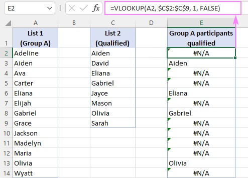
8. Leveraging VLOOKUP to Retrieve Values from a Third Column
One of the most powerful applications of VLOOKUP is to compare two columns and return a corresponding value from a third column in the table array.
8.1 Basic Formula:
=VLOOKUP(A2, $B$2:$C$100, 2, FALSE)
In this formula:
- A2 is the lookup value from List 1.
- $B$2:$C$100 is the table array, where Column B contains List 2 (the values to compare against), and Column C contains the values you want to return.
- 2 is the column index number, indicating that you want to return values from the second column in the table array (Column C).
- FALSE specifies an exact match.
8.2 Handling Errors:
To handle errors, use the IFNA function:
=IFNA(VLOOKUP(A2, $B$2:$C$100, 2, FALSE), "Not Available")
This will return “Not Available” if a match is not found.
9. Alternative Methods: INDEX MATCH and XLOOKUP for Comparison
While VLOOKUP is a valuable tool, INDEX MATCH and XLOOKUP offer more flexible and powerful alternatives for data comparison.
9.1 INDEX MATCH:
INDEX and MATCH can be combined to perform lookups. This combination is more flexible than VLOOKUP because it doesn’t require the lookup value to be in the first column of the table array.
=INDEX($C$2:$C$100, MATCH(A2, $B$2:$B$100, 0))
In this formula:
$C$2:$C$100is the range containing the values you want to return.MATCH(A2, $B$2:$B$100, 0)finds the position of A2 in the range$B$2:$B$100.- INDEX then returns the value from
$C$2:$C$100at the position found by MATCH.
9.2 XLOOKUP:
XLOOKUP is the modern successor to VLOOKUP and HLOOKUP, available in Excel 365 and Excel 2021. It offers several advantages, including the ability to look up values to the left and right, and built-in error handling.
=XLOOKUP(A2, $B$2:$B$100, $C$2:$C$100, "Not Found")
In this formula:
- A2 is the lookup value.
$B$2:$B$100is the lookup array (where you want to find the lookup value).$C$2:$C$100is the return array (the values you want to return).- “Not Found” is the value to return if a match is not found.
10. Streamlining Comparison with Specialized Tools
For users who frequently perform data comparison tasks, specialized tools can significantly streamline the process. At COMPARE.EDU.VN, we recommend exploring the following:
- Excel’s Built-in Comparison Features: Excel offers several built-in features for comparing data, such as conditional formatting, data validation, and the “Compare Side by Side” view.
- Third-Party Add-ins: Several third-party add-ins are available for Excel that provide advanced data comparison capabilities, such as identifying duplicates, finding differences, and merging data.
11. Frequently Asked Questions (FAQs) About VLOOKUP Comparison
- Q: Can VLOOKUP compare text values?
- A: Yes, VLOOKUP can compare text values. Ensure that the text values are formatted consistently in both columns to ensure accurate matches.
- Q: How do I handle case sensitivity in VLOOKUP?
- A: VLOOKUP is not case-sensitive by default. To perform a case-sensitive lookup, use the FIND function within an IF statement to check for an exact match.
- Q: Can VLOOKUP compare values in multiple columns?
- A: VLOOKUP can only compare values in the first column of the table array. To compare values in multiple columns, consider using INDEX MATCH with multiple criteria or exploring alternative methods like Power Query.
- Q: What are the limitations of VLOOKUP?
- A: VLOOKUP has several limitations, including the requirement that the lookup value be in the first column of the table array, the inability to look up values to the left, and the lack of built-in error handling. These limitations can be overcome by using INDEX MATCH or XLOOKUP.
12. Conclusion: Mastering Data Comparison with VLOOKUP and COMPARE.EDU.VN
Comparing data in Excel using VLOOKUP is a fundamental skill that can significantly enhance your data analysis capabilities. Whether you’re identifying matches, finding differences, or retrieving corresponding values, VLOOKUP provides a powerful and efficient solution. By mastering the techniques outlined in this guide, you can streamline your data comparison processes and make informed decisions based on accurate and readily available insights.
At COMPARE.EDU.VN, we are dedicated to providing you with the knowledge and resources you need to excel in data analysis. Visit our website at COMPARE.EDU.VN to explore more tutorials, resources, and tools to help you master Excel and other data analysis techniques.
Address: 333 Comparison Plaza, Choice City, CA 90210, United States.
Whatsapp: +1 (626) 555-9090.
Looking for more ways to compare and decide? Let compare.edu.vn be your guide.
Remember, effective data comparison is the key to unlocking valuable insights and driving informed decision-making.