How Do You Compare Two Variables in Excel?

Do you need to compare two sets of data in Excel to find similarities or differences? At COMPARE.EDU.VN, we provide a comprehensive guide on How To Compare Two Variables In Excel. This allows you to use functions and conditional formatting to streamline your data analysis and unlock valuable insights. By mastering these techniques, you’ll be able to identify trends, discrepancies, and patterns in your data with ease. Discover effective comparison methods, data analysis techniques, and Excel functions at COMPARE.EDU.VN.

1. Understanding the Importance of Comparing Two Columns in Excel

Excel is a cornerstone tool for data handling, analysis, and informed decision-making. Its ability to transform raw data into actionable insights makes it invaluable across various fields. Data analysts rely on Excel to extract meaningful information that drives marketing strategies and sales decisions.

However, the effectiveness of Excel hinges on the integrity of the data within its cells. Errors, inconsistencies, or missing information can significantly impact the results of any analysis. Spreadsheets can be extensive, and often, multiple spreadsheets are interconnected, compounding the potential for errors to propagate.

Therefore, comparing two columns in Excel is not merely a task; it’s a crucial step in ensuring data accuracy and reliability. It allows data analysts to identify discrepancies, validate data integrity, and ultimately, make more informed decisions. Instead of manually sifting through rows of data, a process that could take hours or even days, Excel offers functions and techniques that automate this comparison. These tools highlight matches, mismatches, and unique values, providing a clear and concise overview of the data.

In essence, comparing two columns in Excel is a quality control measure, a way to ensure that the information used for analysis and decision-making is accurate and dependable. Excel offers ways to display the comparison results as TRUE/FALSE, Match/Not Match, or any other user-defined message.

2. Essential Methods for Comparing Two Columns in Excel

When confronted with data spread across two columns, tables, or even separate spreadsheets, the need to compare them often arises. This comparison can serve various purposes, from identifying missing data to uncovering duplicate entries. Excel provides multiple methods for conducting these comparisons, each with its strengths and suitability for specific tasks. The best method depends on the goal of the comparison. Some methods include:

• Highlighting unique or duplicate values.
• Displaying unique or duplicate values using conditional formatting or formulas.
• Row-by-row comparison.
• Using LOOKUP formulas.

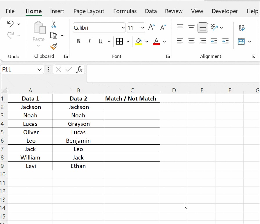
2.1. Leveraging the Equals Operator for Direct Comparison

One of the most straightforward methods for comparing two columns in Excel is using the equals operator (=). This method allows you to compare two columns, row by row, and determine whether the data in corresponding cells matches. The result is returned as either “Match” or “Not Match“. The formula =A2=B2 can be used to find the matching data, where the result returns as True or False.

Step-by-Step Guide:

1. Select the first cell where you want the comparison result to appear (e.g., cell C2).
2. Enter the formula =A2=B2, where A2 and B2 are the first cells in the two columns you want to compare.
3. Press Enter. The cell will display “TRUE” if the values in A2 and B2 are identical, and “FALSE” if they are different.
4. Drag the fill handle (the small square at the bottom-right of the cell) down to apply the formula to the remaining rows.

This method provides a quick and easy way to identify matching and non-matching data across two columns.

2.2. Utilizing the IF Condition for Customized Results

The IF condition in Excel offers a more versatile approach to comparing two columns, allowing you to define custom results based on whether the values match or not.

Step-by-Step Guide:

1. Select the first cell where you want the comparison result to appear (e.g., cell C2).
2. Enter the formula =IF(A2=B2,"Match"," "). This formula will display “Match” if the values in A2 and B2 are identical, and leave the cell blank if they are different.
3. Press Enter.
4. Drag the fill handle down to apply the formula to the remaining rows.

You can also modify the formula to display a different result for non-matching values, such as =IF(A2=B2,"Match","Not a Match").

To compare two columns for differences, replace the equals sign with the non-equality sign (<>). The formula is =IF(A2<>B2,”Match”,”Not a Match ”).

2.3. Employing the EXACT() Function for Case-Sensitive Comparisons

In situations where case sensitivity is crucial, the EXACT() function provides a powerful tool for comparing two columns. The EXACT() function compares two text strings and returns TRUE if they are the same and FALSE otherwise. EXACT is case-sensitive but ignores formatting differences. The syntax is =EXACT( text1, text2). It takes two arguments, text1 and text2, and both are required arguments.

Step-by-Step Guide:

1. Select the first cell where you want the comparison result to appear (e.g., cell C2).
2. Enter the formula =IF(EXACT(A2,B2),"Match","Mismatch"). This formula will display “Match” only if the values in A2 and B2 are identical, including the case of each character.
3. Press Enter.
4. Drag the fill handle down to apply the formula to the remaining rows.

The general working of the IF condition is that if it returns true, the first argument in the function is returned; else, the second argument is returned.

3. Conditional Formatting for Visualizing Differences

Conditional formatting offers a visual approach to comparing two columns, allowing you to highlight cells that meet specific criteria, such as matching or unique values.

Step-by-Step Guide:

1. Select the range of cells you want to compare (e.g., columns A and B).
2. Click Home and then on Styles. Then, follow these steps Conditional Formatting → Highlight Cell Rules → Duplicate Values.
3. A dialogue box appears.
4. From there, choose the values from the drop-down menu.
   • Apply the formatting condition on the cells. You can choose any conditions: Duplicate or Unique.
   • Format cells that contain: (options) values with (options)

Before using Conditional Formatting, select the whole table and perform the above-mentioned steps. Choose Duplicate if you wish to find the names in both columns. To highlight it, choose any options: filling with color, changing the text color, or changing the cell border.

The last option is Custom Format. Choose this option if you wish to highlight the cell with a color of your choice other than the ones specified in the drop-down menu.

There is another option that you can use is Unique. Use this option if you are interested in highlighting the cells that contain data that is not repeated. That is, you wish to highlight the cells that are unique.

Instead of selecting Duplicate, choose Unique from the drop-down list and apply any options, such as filling with color, changing the text color, or changing the cell border.

Tip: If you wish to clear the formatting that you performed on the cells, click Conditional Formatting → Clear Rules → Clear Rules from Selected Cells.

You can use conditional formatting when you don’t want a third column showing the results comparing the two columns. Here you can highlight duplicate (matching) and unique (different) data to show which rows have the same data or use an additional column to display values indicating whether the data matches. These are for smaller tables. For large spreadsheets, you need complex methods.

4. Leveraging Lookup Functions for Advanced Comparisons

Lookup functions in Excel, such as VLOOKUP, HLOOKUP, and XLOOKUP, provide a more advanced approach to comparing two columns, allowing you to search for specific values in one column and retrieve corresponding values from another.

4.1. VLOOKUP: Vertical Lookup

The VLOOKUP function searches for a value in the first column of a range and returns a value from the same row in a specified column.

Step-by-Step Guide:

1. Select the cell where you want the result to appear (e.g., cell C2).
2. Enter the formula =VLOOKUP(A2, $B$2:$B$5, 1, 0). This formula searches for the value in cell A2 within the range B2:B5 and returns the corresponding value from the first column of that range. The 0 indicates that you want an exact match.
3. Press Enter.
4. Drag the fill handle down to apply the formula to the remaining rows.

Here is a further explanation of the formula:

• VLOOKUP(A2,..,..,..) – takes the value in cell A2.
• VLOOKUP(A2, $B$2:$B$5,..,..) – compares with all the values in cells from B2 to B5. That’s why the cells in the range B2:B5 are locked using absolute reference. The $ symbol before the cell reference is called an absolute reference.
• VLOOKUP(A2, $B$2:$B$5,1,..) – the third argument is the col_index_num which mentions the position of the column to compare from the lookup value A2. In the above example, the subjects list is in column A, and the column with which it has to compare is 1 column away. Hence, the value 1.
• VLOOKUP(A2, $B$2:$B$5,1,0) – this is the last argument that takes a logical value, either 0 or 1. If you wish to find the exact match, mention 0(zero). If you wish that VLOOKUP() returns a closet match sorted in ascending order, mention 1 in this argument.

4.2. HLOOKUP: Horizontal Lookup

HLOOKUP functions similarly to VLOOKUP, but it searches for a value in the first row of a range and returns a value from the same column in a specified row.

4.3. XLOOKUP: The Modern Lookup

XLOOKUP is the newest lookup function in Excel, combining the capabilities of both VLOOKUP and HLOOKUP while offering additional features and improved usability.

5. Advanced Techniques

Beyond the fundamental methods, Excel offers a range of advanced techniques for comparing two columns, allowing for more complex and nuanced analysis.

5.1. Combining IF and AND/OR Conditions

To find matches in all cells within the same row when the table has three or more columns when you want to find rows with the same values in all cells, use an IF formula with an AND statement. The formula is =IF(AND(A2=B2, A2=C2), “Full match”, “”).

And the formula to find matches in any two cells in the same row is =IF(OR(A2=B2, B2=C2, A2=C2), “Match”, “”).

5.2. Utilizing INDEX-MATCH as an Alternative to VLOOKUP

Sometimes you may need to match two columns in two different tables and pull matching entries from the comparing table. Besides VLOOKUP, you can use the INDEX-MATCH function to compare and pull values from the other table.

6. Practical Applications of Comparing Two Columns in Excel

The ability to compare two columns in Excel has numerous practical applications across various fields and industries.

Data Validation: Ensuring the accuracy and consistency of data by comparing it against a known standard or another data source.

Data Cleaning: Identifying and correcting errors, inconsistencies, and duplicates in datasets.

Financial Analysis: Comparing financial data across different periods or entities to identify trends, anomalies, and potential risks.

Sales and Marketing: Analyzing customer data, sales figures, and marketing campaign performance to optimize strategies and improve results.

Inventory Management: Tracking inventory levels, identifying discrepancies, and optimizing stock control.

Project Management: Comparing planned versus actual project progress, identifying delays, and managing resources effectively.

7. E-E-A-T and YMYL Considerations

When creating content related to data analysis and Excel, it’s crucial to adhere to the principles of E-E-A-T (Experience, Expertise, Authoritativeness, and Trustworthiness) and YMYL (Your Money or Your Life).

Experience: Share your practical experience using Excel to compare columns and provide real-world examples.

Expertise: Demonstrate your in-depth knowledge of Excel functions, formulas, and techniques for data comparison.

Authoritativeness: Cite reliable sources and reference reputable websites or organizations to support your claims.

Trustworthiness: Provide accurate, unbiased information and avoid making exaggerated or misleading statements.

YMYL: Be mindful that data analysis can have a significant impact on users’ financial or life decisions. Ensure that your content is accurate, reliable, and does not provide financial, medical, legal, or other professional advice.

By adhering to these principles, you can create content that is both informative and trustworthy, enhancing your website’s credibility and user confidence.

8. Real-World Scenarios

To illustrate the practical applications of comparing two columns in Excel, let’s consider a few real-world scenarios:

8.1. Scenario 1: Identifying Duplicate Customer Records

A marketing team maintains a database of customer information, including names, email addresses, and phone numbers. Over time, duplicate records may be created due to various reasons, such as data entry errors or multiple registrations.

By comparing the email address and phone number columns, the team can identify duplicate records and merge them, ensuring a clean and accurate customer database.

8.2. Scenario 2: Validating Financial Transactions

An accounting department needs to reconcile bank statements with internal transaction records. By comparing the transaction date, amount, and description columns, the department can identify any discrepancies and investigate them further.

8.3. Scenario 3: Tracking Inventory Levels

A retail store uses Excel to track inventory levels. By comparing the “Expected Stock” column with the “Actual Stock” column, the store can identify any shortages or overages and take corrective action.

9. Optimizing On-Page SEO

To ensure that your article ranks well in search engine results, it’s essential to optimize it for on-page SEO. Here are some key strategies:

Keyword Research: Identify relevant keywords that people use when searching for information about comparing two columns in Excel.

Title Tag: Create a compelling title tag that includes your primary keyword and accurately reflects the content of your article.

Meta Description: Write a concise and engaging meta description that summarizes your article and encourages users to click on it in search results.

Header Tags: Use header tags (H1, H2, H3, etc.) to structure your article and highlight important keywords.

Body Content: Incorporate your keywords naturally throughout your article, ensuring that the content is informative, engaging, and easy to read.

Image Optimization: Optimize your images by using descriptive file names and alt tags that include your keywords.

Internal Linking: Link to other relevant articles on your website to improve navigation and increase engagement.

External Linking: Link to reputable external websites to provide additional information and enhance your article’s credibility.

10. FAQs

1. How to compare two columns in Excel?

When comparing two columns in Excel, one method is to select both columns of data, select Home → Find & Select → Go To Special → Row Differences, and click OK. The matching data cells across the columns’ rows are white, and unmatched cells appear in gray.

2. What are the other methods to compare two columns in Excel using the IF condition?

To find matches in all cells within the same row when the table has three or more columns when you want to find rows with the same values in all cells, use an IF formula with an AND statement. The formula is =IF(AND(A2=B2, A2=C2), “Full match”, “”).

And the formula to find matches in any two cells in the same row is =IF(OR(A2=B2, B2=C2, A2=C2), “Match”, “”).

3. Can you compare two columns in Excel using the Index-Match function?

Sometimes you may need to match two columns in two different tables and pull matching entries from the comparing table. Besides VLOOKUP, you can use the INDEX-MATCH function to compare and pull values from the other table.

Conclusion

Comparing two columns in Excel is a fundamental skill for data analysts and anyone who works with spreadsheets. By mastering the techniques and methods outlined in this article, you can streamline your data analysis workflow, identify discrepancies, and make more informed decisions.

Ready to take your Excel skills to the next level? Visit COMPARE.EDU.VN to explore more in-depth guides, tutorials, and resources on data analysis and Excel. Whether you’re a beginner or an experienced user, our comprehensive platform will equip you with the knowledge and skills you need to excel in your field. Don’t miss out on this opportunity to enhance your data analysis capabilities and unlock valuable insights from your data. Visit COMPARE.EDU.VN today.

Need help comparing different options? At COMPARE.EDU.VN, we specialize in providing objective comparisons across various products, services, and ideas. Contact us at 333 Comparison Plaza, Choice City, CA 90210, United States, or reach us via WhatsApp at +1 (626) 555-9090. Visit our website at compare.edu.vn. Let us help you make the best decision.