How To Compare Two Values In Excel Sheet?

Comparing two values in an Excel sheet can be easily achieved with various built-in functions and techniques. COMPARE.EDU.VN offers in-depth guides and tutorials to help you master these methods. Learn to identify matches, differences, and unique entries efficiently using formulas like IF, COUNTIF, and VLOOKUP, or explore user-friendly tools for a streamlined comparison process, ensuring data accuracy and informed decision-making with Excel. Dive into Excel comparisons with confidence, exploring techniques like conditional formatting, exact matching, and dealing with multiple columns.

1. Understanding the Basics of Comparing Values in Excel

Excel is a powerful tool for data analysis, and one of its most common uses is comparing values. Whether you’re comparing sales figures, inventory levels, or any other type of data, Excel provides a variety of functions and techniques to help you quickly and accurately identify similarities and differences. Mastering these techniques is crucial for efficient data management and informed decision-making. Let’s explore the fundamental methods for comparing values in Excel sheets.

1.1. Why Compare Values in Excel?

Comparing values in Excel is essential for various reasons. It helps in identifying trends, detecting discrepancies, and making informed decisions based on data. Whether you’re auditing financial statements, analyzing sales data, or managing inventory, the ability to compare values accurately is crucial. Here are some key reasons:

Data Validation: Ensuring data accuracy by comparing values across different sources or columns.
Trend Analysis: Identifying patterns and trends by comparing data over time.
Decision Making: Making informed decisions based on comparative analysis.
Error Detection: Spotting discrepancies and errors in datasets.
Performance Tracking: Monitoring performance metrics by comparing current values against targets or past performance.

1.2. Key Excel Functions for Comparison

Excel offers several built-in functions that facilitate value comparison. Understanding these functions is key to performing effective data analysis. Here are some of the most commonly used functions:

IF Function: This function allows you to perform logical tests and return different values based on whether the test is true or false. It’s fundamental for comparing values and making decisions based on the comparison.
COUNTIF Function: This function counts the number of cells within a range that meet a given criteria. It’s useful for identifying the frequency of certain values and comparing lists.
VLOOKUP Function: This function searches for a value in the first column of a range and returns a value in the same row from another column. It’s commonly used to compare data between two different tables.
MATCH Function: This function searches for a specified item in a range of cells, and then returns the relative position of that item in the range. It’s useful for locating specific values in a list.
EXACT Function: This function checks if two text strings are exactly the same, including case. It’s particularly useful for case-sensitive comparisons.
ISERROR Function: This function checks whether a value is an error and returns TRUE or FALSE. It’s often used in conjunction with other functions to handle potential errors during comparison.
AND Function: This function checks whether all conditions in a test are TRUE.
OR Function: This function checks whether any of the conditions in a test are TRUE.

1.3. Setting Up Your Excel Sheet for Comparison

Before diving into formulas, it’s important to set up your Excel sheet in a way that makes comparison easier. Here are some tips:

Organize Your Data: Ensure your data is well-organized in columns and rows with clear headers.
Use Consistent Formatting: Apply consistent formatting to your data to avoid errors during comparison.
Freeze Panes: Freeze the top row or first column to keep headers visible when scrolling through large datasets.
Use Tables: Convert your data range into an Excel table for easier referencing and automatic formula adjustments.
Data Validation: Use data validation to restrict the type of data that can be entered into cells, ensuring consistency.

1.4. Basic Comparison Operators

Understanding basic comparison operators is crucial for writing effective Excel formulas. These operators allow you to define the conditions for your comparisons. Here are the main comparison operators:

= (Equal to): Checks if two values are equal.
<> (Not equal to): Checks if two values are not equal.
> (Greater than): Checks if a value is greater than another.
< (Less than): Checks if a value is less than another.
>= (Greater than or equal to): Checks if a value is greater than or equal to another.
<= (Less than or equal to): Checks if a value is less than or equal to another.

2. Comparing Two Columns Row by Row

Comparing two columns row by row is a common task in Excel data analysis. It involves checking the values in corresponding rows of two columns and identifying matches or differences. This method is useful for validating data, identifying discrepancies, and performing detailed comparisons. Let’s explore how to accomplish this using the IF function and other techniques.

2.1. Using the IF Function for Basic Comparison

The IF function is a versatile tool for comparing two columns row by row. It allows you to perform a logical test and return different values based on the outcome.

Formula for Matches

To find cells within the same row having the same content, use the following formula:

=IF(A2=B2,"Match","")

In this formula:

A2 and B2 are the first two cells you are comparing.
"Match" is the value returned if the condition A2=B2 is true.
"" is the value returned if the condition is false (empty string).

Formula for Differences

To find cells in the same row with different values, simply replace the equals sign with the non-equality sign (<>):

=IF(A2<>B2,"No match","")

In this formula:

A2 and B2 are the cells being compared.
"No match" is the value returned if the condition A2<>B2 is true.
"" is the value returned if the condition is false.

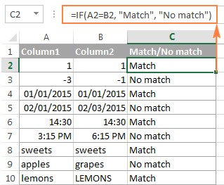
Combining Matches and Differences

You can also combine the logic to find both matches and differences with a single formula:

=IF(A2=B2,"Match","No match")

Or:

=IF(A2<>B2,"No match","Match")

These formulas handle numbers, dates, times, and text strings equally well.

2.2. Case-Sensitive Comparisons Using the EXACT Function

The IF function ignores case when comparing text values. If you need to perform a case-sensitive comparison, use the EXACT function.

Formula for Case-Sensitive Matches

=IF(EXACT(A2,B2),"Match","")

In this formula:

EXACT(A2, B2) returns TRUE if the values in A2 and B2 are exactly the same (including case), and FALSE otherwise.
"Match" is the value returned if the condition is true.
"" is the value returned if the condition is false.

Formula for Case-Sensitive Differences

=IF(EXACT(A2,B2),"Match","Unique")

In this formula, "Unique" is returned if the values are not exactly the same.

2.3. Using Conditional Formatting to Highlight Matches and Differences

Conditional formatting can be used to visually highlight matches and differences between two columns.

Highlighting Matches

Select the cells you want to highlight in column A.
Go to Conditional Formatting > New Rule > Use a formula to determine which cells to format.
Enter the formula =$B2=$A2.
Choose a formatting style (e.g., fill color).

Highlighting Differences

Select the cells you want to highlight in column A.
Go to Conditional Formatting > New Rule > Use a formula to determine which cells to format.
Enter the formula =$B2<>$A2.
Choose a formatting style.

2.4. Using Advanced Filter to Compare Two Columns

Excel’s Advanced Filter can also be used to compare two columns.

Filtering Matches

Select your data range, including headers.
Go to Data > Advanced.
Set the Criteria range to include the headers of the two columns you want to compare.
In the row below the headers in the criteria range, enter the formula =$A2=$B2.
Click OK to filter the matches.

Filtering Differences

Select your data range, including headers.
Go to Data > Advanced.
Set the Criteria range to include the headers of the two columns.
In the row below the headers in the criteria range, enter the formula =$A2<>$B2.
Click OK to filter the differences.

3. Comparing Multiple Columns for Matches

When working with larger datasets, you may need to compare multiple columns to identify matches or unique entries. Excel provides functions and techniques to handle these complex comparisons efficiently. Let’s explore how to compare multiple columns for matches within the same row.

3.1. Finding Matches in All Cells Within the Same Row

If you want to find rows where all cells in multiple columns have the same value, you can use the IF function with the AND statement or the COUNTIF function.

Using IF with AND

For a table with three columns (A, B, and C), the formula is:

=IF(AND(A2=B2,A2=C2),"Full match","")

In this formula:

AND(A2=B2, A2=C2) checks if the value in A2 is equal to both B2 and C2.
"Full match" is returned if the condition is true.
"" is returned if the condition is false.

Using COUNTIF

For a more elegant solution, especially with many columns, use the COUNTIF function:

=IF(COUNTIF($A2:$E2,$A2)=5,"Full match","")

In this formula:

$A2:$E2 is the range of columns you are comparing.
$A2 is the criteria (the value in the first column of the range).
5 is the number of columns you are comparing.
"Full match" is returned if the count equals the number of columns.
"" is returned if the count does not equal the number of columns.

3.2. Finding Matches in Any Two Cells in the Same Row

If you want to identify rows where any two or more cells have the same values, use the IF function with the OR statement or a combination of COUNTIF functions.

Using IF with OR

For a table with three columns (A, B, and C), the formula is:

=IF(OR(A2=B2,B2=C2,A2=C2),"Match","")

In this formula:

OR(A2=B2, B2=C2, A2=C2) checks if any two cells have the same value.
"Match" is returned if the condition is true.
"" is returned if the condition is false.

Using COUNTIF Combinations

For tables with many columns, combining COUNTIF functions can be more efficient:

=IF(COUNTIF(B2:D2,A2)+COUNTIF(C2:D2,B2)+(C2=D2)=0,"Unique","Match")

In this formula:

COUNTIF(B2:D2,A2) counts how many columns have the same value as in the first column (A2).
COUNTIF(C2:D2,B2) counts how many of the remaining columns are equal to the second column (B2).
(C2=D2) checks if the last two columns are equal.
=0 checks if the total count is zero (meaning no matches were found).
"Unique" is returned if no matches are found.
"Match" is returned if any matches are found.

3.3. Highlighting Row Differences and Matches in Multiple Columns

Conditional formatting and the “Go To Special” feature can be used to highlight row differences and matches in multiple columns.

Highlighting Row Matches

To highlight rows that have identical values in all columns, create a conditional formatting rule based on one of the following formulas:

=AND($A2=$B2,$A2=$C2)

Or:

=COUNTIF($A2:$C2,$A2)=3

Where A2, B2, and C2 are the top-most cells and 3 is the number of columns to compare.

Highlighting Row Differences

To quickly highlight cells with different values in each individual row, use Excel’s “Go To Special” feature.

Select the range of cells you want to compare.
On the Home tab, go to Editing group, and click Find & Select > Go To Special….
Select Row differences and click OK.
The cells whose values are different from the comparison cell in each row are colored.

4. Comparing Two Lists for Matches and Differences

Comparing two lists is a common requirement in data analysis. Whether you need to identify common entries, find unique items, or validate data, Excel offers several techniques to accomplish this task efficiently. Let’s explore how to compare two lists in Excel for matches and differences.

4.1. Identifying Values in One Column But Not in Another

To find values that are in column A but not in column B, you can use the COUNTIF function within an IF formula.

=IF(COUNTIF($B:$B,$A2)=0,"No match in B","")

In this formula:

COUNTIF($B:$B,$A2) counts how many times the value in A2 appears in column B.
=0 checks if the count is zero, indicating no match was found.
"No match in B" is returned if no match is found.
"" is returned if a match is found.

Tip: If your table has a fixed number of rows, specify a certain range (e.g., $B2:$B10) rather than the entire column ($B:$B) for the formula to work faster on large datasets.

4.2. Alternative Formulas Using ISERROR and MATCH

You can also achieve the same result using an IF formula with the embedded ISERROR and MATCH functions:

=IF(ISERROR(MATCH($A2,$B$2:$B$10,0)),"No match in B","")

Or, by using the following array formula (remember to press Ctrl + Shift + Enter to enter it correctly):

=IF(SUM(--($B$2:$B$10=$A2))=0,"No match in B","")

4.3. Identifying Both Matches and Differences in a Single Formula

If you want a single formula to identify both matches (duplicates) and differences (unique values), put some text for matches in the empty double quotes ("") in any of the above formulas. For example:

=IF(COUNTIF($B:$B,$A2)=0,"No match in B","Match in B")

4.4. Highlighting Unique Entries in Each List

Conditional formatting can be used to highlight unique entries in each list.

Select the range of cells in List 1 (column A).
Go to Conditional Formatting > New Rule > Use a formula to determine which cells to format.
Enter the formula =COUNTIF($C$2:$C$5,$A2)=0.
Choose a formatting style.

Repeat for List 2 (column C), using the formula =COUNTIF($A$2:$A$6,$C2)=0.

4.5. Highlighting Matches (Duplicates) Between Two Columns

To highlight matches (duplicates) between two columns, adjust the COUNTIF formulas so that they find the matches rather than differences.

Select the range of cells in List 1 (column A).
Go to Conditional Formatting > New Rule > Use a formula to determine which cells to format.
Enter the formula =COUNTIF($C$2:$C$5,$A2)>0.
Choose a formatting style.

Repeat for List 2 (column C), using the formula =COUNTIF($A$2:$A$6,$C2)>0.

5. Pulling Matching Entries from Another List

Sometimes, you may need to not only match two columns but also pull matching entries from the lookup table. Excel provides functions like VLOOKUP, INDEX MATCH, and XLOOKUP to accomplish this task. Let’s explore how to use these functions to pull matching entries from another list.

5.1. Using VLOOKUP to Pull Matching Entries

The VLOOKUP function searches for a value in the first column of a range and returns a value in the same row from another column.

=VLOOKUP(D2,$A$2:$B$6,2,FALSE)

In this formula:

D2 is the lookup value (the value you want to find in the first column of the range).
$A$2:$B$6 is the range in which to search.
2 is the column number in the range from which to return a value.
FALSE specifies an exact match.

5.2. Using INDEX MATCH to Pull Matching Entries

The INDEX MATCH combination is a more powerful and versatile alternative to VLOOKUP.

=INDEX($B$2:$B$6,MATCH($D2,$A$2:$A$6,0))

In this formula:

$B$2:$B$6 is the range from which to return a value.
MATCH($D2,$A$2:$A$6,0) finds the row number where the lookup value is found in the range $A$2:$A$6.
0 specifies an exact match.

5.3. Using XLOOKUP to Pull Matching Entries

The XLOOKUP function is available in Excel 2021 and Excel 365 and is a more modern and flexible alternative to VLOOKUP and INDEX MATCH.

=XLOOKUP(D2,$A$2:$A$6,$B$2:$B$6)

In this formula:

D2 is the lookup value.
$A$2:$A$6 is the lookup array.
$B$2:$B$6 is the return array.

For more information, please see How to compare two columns using VLOOKUP.

6. Formula-Free Comparison: Using Compare Two Tables Add-in

While Excel offers various functions and techniques for comparing values, a formula-free solution can streamline the process and make it more accessible to users of all skill levels. The Compare Two Tables add-in, part of the Ultimate Suite, provides an intuitive way to compare two lists or tables without writing complex formulas.

6.1. Overview of the Compare Two Tables Add-in

The Compare Two Tables add-in simplifies the process of comparing data in Excel. It allows you to compare two tables or lists by any number of columns and both identify matches/differences and highlight them. This add-in is particularly useful for users who prefer a visual, step-by-step approach to data comparison.

6.2. Step-by-Step Guide to Using the Add-in

To compare two lists using the Compare Two Tables add-in, follow these steps:

Start the Add-in: Click the Compare Tables button on the Ablebits Data tab.
Select the First List: Select the first column/list and click Next. This is your Table 1.
Select the Second List: Select the second column/list and click Next. This is your Table 2, and it can reside in the same or different worksheet or even in another workbook.
Choose Data Type: Choose what kind of data to look for:
- Duplicate values (matches) – the items that exist in both lists.
- Unique values (differences) – the items that are present in list 1, but not in list 2.
Select Columns for Comparison: Select the columns for comparison. In bigger tables, you can select several column pairs to compare by.
Choose How to Deal with Found Items: In the final step, you choose how to deal with the found items and click Finish. A few different options are available here:
- Highlight with color – shades matches or differences in the selected color (like Excel conditional formatting does).
- Identify in the Status column – inserts the Status column with the “Duplicate” or “Unique” labels (like IF formulas do).

6.3. Highlighting Matches and Differences with the Add-in

The add-in allows you to highlight matches and differences in a selected color, similar to Excel’s conditional formatting. This visual representation makes it easy to identify common and unique entries between the two lists.

6.4. Identifying Matches and Differences with the Status Column

The add-in can insert a Status column with labels such as “Duplicate” or “Unique,” similar to using IF formulas. This provides a clear, text-based indication of whether each entry is a match or a unique value.

7. Advanced Tips and Tricks for Efficient Comparison

To enhance your data comparison skills in Excel, consider these advanced tips and tricks that can streamline your workflow and improve accuracy.

7.1. Using Array Formulas for Complex Comparisons

Array formulas are powerful tools for performing complex calculations on multiple values simultaneously. They can be used to compare entire ranges of cells and return results based on multiple criteria.

Comparing Two Ranges for Exact Matches

To check if two ranges are exactly the same, you can use the following array formula:

=AND(A1:A5=B1:B5)

Enter this formula by pressing Ctrl + Shift + Enter. The formula returns TRUE if all corresponding cells in the two ranges are equal, and FALSE otherwise.

Counting Differences Between Two Ranges

To count the number of differences between two ranges, use the following array formula:

=SUM(--(A1:A5<>B1:B5))

Enter this formula by pressing Ctrl + Shift + Enter. The formula returns the number of cells where the values in the two ranges are different.

7.2. Using Named Ranges for Easier Formula Management

Named ranges make formulas easier to read and manage. Instead of using cell references like A1:A10, you can define a name for that range and use the name in your formulas.

Defining a Named Range

Select the range of cells you want to name.
Go to the Formulas tab and click Define Name.
Enter a name for the range and click OK.

Using Named Ranges in Formulas

Once you’ve defined a named range, you can use it in your formulas:

=SUM(SalesData)

Where “SalesData” is the name of the range containing your sales figures.

7.3. Combining Multiple Criteria in Comparisons

You can combine multiple criteria in your comparisons using the AND and OR functions.

Using AND for Multiple Criteria

To check if multiple conditions are true, use the AND function:

=IF(AND(A2>10,B2<20),"Valid","Invalid")

This formula checks if the value in A2 is greater than 10 and the value in B2 is less than 20.

Using OR for Multiple Criteria

To check if at least one of multiple conditions is true, use the OR function:

=IF(OR(A2>10,B2<20),"Valid","Invalid")

This formula checks if the value in A2 is greater than 10 or the value in B2 is less than 20.

7.4. Handling Errors in Comparison Formulas

Errors can occur in comparison formulas due to various reasons, such as blank cells or incorrect data types. Use the IFERROR function to handle these errors gracefully.

Using IFERROR to Handle Errors

=IFERROR(VLOOKUP(D2,$A$2:$B$6,2,FALSE),"Not Found")

This formula attempts to perform a VLOOKUP and returns “Not Found” if an error occurs.

8. Common Mistakes to Avoid When Comparing Values

When comparing values in Excel, several common mistakes can lead to inaccurate results. Being aware of these pitfalls can help you avoid errors and ensure your comparisons are reliable.

8.1. Ignoring Case Sensitivity

Excel’s default comparison is not case-sensitive. If you need to perform a case-sensitive comparison, use the EXACT function.

Example of Case-Sensitive Comparison

=IF(EXACT(A2,B2),"Match","No Match")

This formula distinguishes between “apple” and “Apple.”

8.2. Not Accounting for Different Data Types

Excel treats different data types (e.g., numbers, text, dates) differently. Ensure that the data types you are comparing are consistent.

Converting Data Types

Use functions like VALUE, TEXT, and DATE to convert data types:

=VALUE(A2) converts text to a number.
=TEXT(A2,"yyyy-mm-dd") converts a date to text.

8.3. Overlooking Trailing Spaces

Trailing spaces can cause comparison errors. Use the TRIM function to remove leading and trailing spaces from text values.

Removing Trailing Spaces

=IF(TRIM(A2)=TRIM(B2),"Match","No Match")

This formula removes trailing spaces before comparing the values.

8.4. Using Incorrect Cell References

Using incorrect cell references can lead to comparisons of the wrong values. Double-check your formulas to ensure you are referencing the correct cells.

Absolute vs. Relative References

Use absolute references ($A$2) when you want a cell reference to remain constant, and relative references (A2) when you want it to adjust based on the formula’s position.

8.5. Not Validating Data Before Comparison

Failing to validate data before comparison can lead to errors. Use data validation to ensure that the data you are comparing is accurate and consistent.

Setting Up Data Validation

Select the cells you want to validate.
Go to Data > Data Validation.
Set the validation criteria (e.g., whole number, decimal, list, date).

9. Real-World Examples of Comparing Values in Excel

To illustrate the practical applications of comparing values in Excel, let’s explore some real-world examples across different industries and scenarios.

9.1. Financial Analysis: Budget vs. Actuals

In financial analysis, comparing budgeted amounts against actual expenditures is crucial for monitoring financial performance.

Scenario

A company wants to compare its monthly budget against actual spending to identify variances.

Steps

Create a table with columns for Budgeted Amount and Actual Amount for each expense category.
Use the formula =IF(B2=A2,"Match","No Match") to compare the budgeted amount against the actual amount for each category.
Use conditional formatting to highlight variances above a certain threshold.
Calculate the variance percentage using the formula =(B2-A2)/A2.

9.2. Inventory Management: Stock Levels vs. Reorder Points

In inventory management, comparing current stock levels against reorder points is essential for maintaining optimal inventory levels.

Scenario

A retail store wants to compare its current stock levels against reorder points to identify items that need to be reordered.

Steps

Create a table with columns for Item Name, Stock Level, and Reorder Point.
Use the formula =IF(B2<C2,"Reorder","OK") to determine if the stock level is below the reorder point.
Use conditional formatting to highlight items that need to be reordered.
Calculate the quantity to reorder using the formula =C2-B2.

9.3. Sales Analysis: Sales Targets vs. Actual Sales

In sales analysis, comparing sales targets against actual sales figures is critical for evaluating sales performance.

Scenario

A sales manager wants to compare the sales targets of each salesperson against their actual sales figures to assess performance.

Steps

Create a table with columns for Salesperson, Sales Target, and Actual Sales.
Use the formula =IF(B2=A2,"Match","No Match") to compare the sales target against the actual sales for each salesperson.
Use conditional formatting to highlight salespeople who have met or exceeded their sales targets.
Calculate the achievement percentage using the formula =(B2-A2)/A2.

9.4. Project Management: Planned vs. Actual Start and End Dates

In project management, comparing planned start and end dates against actual dates is essential for tracking project progress.

Scenario

A project manager wants to compare the planned start and end dates of each task against the actual dates to identify delays.

Steps

Create a table with columns for Task Name, Planned Start Date, Actual Start Date, Planned End Date, and Actual End Date.
Use the formula =IF(C2=B2,"Match","No Match") to compare the planned start date against the actual start date for each task.
Use the formula =IF(E2=D2,"Match","No Match") to compare the planned end date against the actual end date for each task.
Use conditional formatting to highlight tasks that are delayed.
Calculate the delay in days using the formula =C2-B2.

10. Resources for Further Learning

To continue expanding your knowledge of comparing values in Excel, consider exploring these resources for further learning.

10.1. Microsoft Excel Documentation

Microsoft provides comprehensive documentation on Excel functions and features. This is a great resource for understanding the syntax and usage of various comparison functions.

10.2. Online Courses and Tutorials

Platforms like Coursera, Udemy, and LinkedIn Learning offer a wide range of Excel courses, including those focused on data analysis and comparison techniques.

10.3. Excel Blogs and Forums

Many Excel blogs and forums provide tips, tricks, and solutions to common problems. These can be valuable resources for learning from experienced Excel users.

10.4. Books on Excel Data Analysis

Several books cover Excel data analysis in detail, including chapters on data comparison and validation. These books can provide a more structured and in-depth learning experience.

Comparing values in Excel is a fundamental skill for data analysis and decision-making. By mastering the functions, techniques, and tips discussed in this guide, you can efficiently compare data, identify trends, and make informed decisions based on accurate analysis. Remember to visit COMPARE.EDU.VN for more detailed guides and comparisons to enhance your Excel skills.

Ready to take your Excel skills to the next level? Visit compare.edu.vn today to find comprehensive guides and comparisons that will help you master data analysis and make informed decisions. Contact us at 333 Comparison Plaza, Choice City, CA 90210, United States or Whatsapp: +1 (626) 555-9090.

FAQ: Comparing Values in Excel

1. How do I compare two columns in Excel to find matches?

Use the IF and COUNTIF functions. For example, =IF(COUNTIF($B:$B, A2)>0, "Match", "No Match") compares the value in cell A2 against column B.

2. Can I perform a case-sensitive comparison in Excel?

Yes, use the EXACT function. For example, =IF(EXACT(A2, B2), "Match", "No Match") performs a case-sensitive comparison between cells A2 and B2.

3. How can I highlight matches between two columns?

Use conditional formatting with a formula like =$A2=$B2 to highlight matches in column A based on column B.

4. What is the best way to compare multiple columns for identical values?

Use the AND function or the COUNTIF function. For example, =IF(AND(A2=B2, A2=C2), "Match", "No Match") or =IF(COUNTIF($A2:$C2, $A2)=3, "Match", "No Match").

5. How do I find unique values in one column that are not in another?

Use the COUNTIF function. For example, =IF(COUNTIF($B:$B, A2)=0, "Unique", "") identifies values in column A that are not in column B.

6. What is VLOOKUP used for in comparing values?

VLOOKUP is used to find a value in one column and return a corresponding value from another column in a different table. It’s useful for pulling matching entries.

7. How can I handle errors in comparison formulas?

Use the IFERROR function. For example, =IFERROR(VLOOKUP(A2, $B:$C, 2, FALSE), "Not Found") returns “Not Found” if VLOOKUP encounters an error.

8. Is there a formula-free way to compare two columns in Excel?

Yes, you can use add-ins like the “Compare Two Tables” add-in from Ablebits Ultimate Suite, which offers a visual, step-by-step approach.