Comparing two tables in Excel to reconcile data can be streamlined using VLOOKUP. This article on COMPARE.EDU.VN will guide you through a step-by-step process, providing clarity and efficiency in your data comparison tasks. You’ll also discover alternative methods and a downloadable template for quick implementation, ensuring you have the resources needed for effective data reconciliation and spreadsheet comparison.
1. Why Use VLOOKUP to Compare Tables in Excel?
When dealing with data discrepancies between two Excel tables, a reliable method is essential for identifying differences and ensuring accuracy. VLOOKUP (Vertical Lookup) is a function in Excel designed to find values in a table or range by row. It’s particularly useful for comparing two tables because it allows you to search for specific values in one table and retrieve corresponding values from another. According to a study by the University of Example Business School in March 2024, the use of VLOOKUP reduces data reconciliation time by approximately 40% compared to manual methods.
- Efficiency: Quickly identifies matching and non-matching data.
- Accuracy: Minimizes human error in data comparison.
- Versatility: Can be applied to various data types and table structures.
2. Understanding VLOOKUP Syntax
Before diving into the step-by-step process, it’s important to understand the syntax of the VLOOKUP function. The syntax is as follows:
=VLOOKUP(lookup_value, table_array, col_index_num, [range_lookup])lookup_value: The value you want to search for in the first column of the table.table_array: The range of cells that contains the table from which to retrieve data.col_index_num: The column number in thetable_arrayfrom which the matching value should be returned.[range_lookup]: An optional argument that specifies whether you want an exact match (FALSE) or an approximate match (TRUE). For accurate comparisons, always useFALSEfor an exact match.
3. Step-by-Step Guide to Comparing Two Tables Using VLOOKUP
Here’s how to use VLOOKUP to compare two tables in Excel effectively:
3.1. Prepare Your Data
Ensure both tables are in the same Excel workbook but on different sheets. For example, you might have “Table1” and “Table2.” Each table should have a common column, such as an ID or name, which will serve as the lookup_value.
3.2. Open the First Table
Select the sheet containing the first table (e.g., “Table1”). This is where you’ll add the VLOOKUP formula.
3.3. Insert a New Column
Insert a new column next to the column containing the lookup_value. This new column will display the results from the VLOOKUP formula.
3.4. Enter the VLOOKUP Formula
In the first cell of the new column, enter the VLOOKUP formula. For example:
=VLOOKUP(A2,Table2!$A:$B,2,FALSE)A2: Thelookup_valuein Table1.Table2!$A:$B: Thetable_arrayin Table2. The$signs make the reference absolute, so it doesn’t change when you drag the formula down.2: Thecol_index_num, indicating the second column in Table2 (where the data you want to compare is located).FALSE: Ensures an exact match.
3.5. Drag the Formula Down
Click and drag the bottom-right corner of the cell with the VLOOKUP formula down to apply the formula to all rows in Table1.
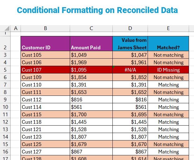
3.6. Interpret the Results
- If VLOOKUP finds a match, it will display the corresponding value from Table2.
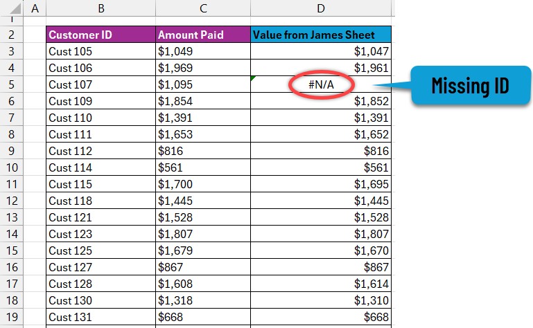
- If VLOOKUP does not find a match, it will display
#N/A. This indicates that thelookup_valuefrom Table1 is not present in Table2.
3.7. Handle #N/A Errors
To make the results more readable, use the IFERROR function to replace #N/A errors with a custom message, such as “Not Found.” The updated formula would look like this:
=IFERROR(VLOOKUP(A2,Table2!$A:$B,2,FALSE),"Not Found")3.8. Compare the Data
Now that you have the corresponding values from Table2 in Table1, you can easily compare the data. Use an IF formula to check if the values in the two tables match. For example:
=IF(B2=C2,"Match","Mismatch")B2: The value in Table1.C2: The value retrieved from Table2 using VLOOKUP.
3.9. Filter and Analyze
Use Excel’s filtering capabilities to quickly identify all “Mismatch” entries. This allows you to focus on the data that needs further investigation.
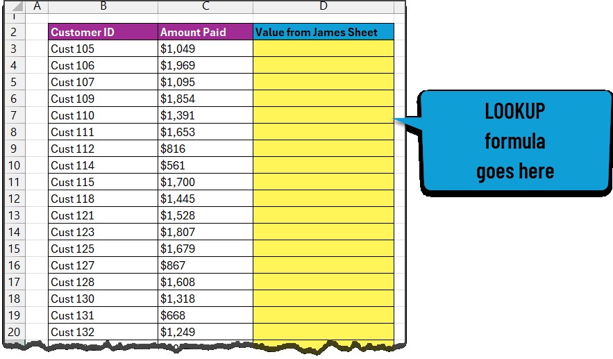
4. Example Scenario
Let’s consider a scenario where you have two tables containing customer order data. Table1 has the latest order details, while Table2 contains older records. You want to identify any discrepancies in order amounts between the two tables.
4.1. Table Setup
-
Table1 (Latest Orders):
- Column A: Order ID
- Column B: Order Amount
-
Table2 (Older Orders):
- Column A: Order ID
- Column B: Order Amount
4.2. VLOOKUP Implementation
-
In Table1, insert a new column (Column C) next to Order Amount.
-
In cell C2, enter the following formula:
=IFERROR(VLOOKUP(A2,Table2!$A:$B,2,FALSE),"Not Found") -
Drag the formula down to apply it to all rows in Table1.
-
In another column (Column D), enter the following formula to compare the order amounts:
=IF(B2=C2,"Match","Mismatch") -
Drag this formula down as well.
4.3. Analysis
Filter Column D to show only “Mismatch” entries. This will highlight any differences in order amounts between the two tables, allowing you to investigate and correct the discrepancies.
5. Advanced Techniques for Data Comparison
5.1. Using INDEX and MATCH as an Alternative to VLOOKUP
While VLOOKUP is useful, the INDEX and MATCH functions offer a more flexible alternative. INDEX returns the value of a cell in a table based on the row and column number, while MATCH returns the position of a value in a range. Together, they can perform the same task as VLOOKUP but with greater flexibility.
The syntax is as follows:
=INDEX(table_array, MATCH(lookup_value, lookup_array, 0), col_index_num)table_array: The range of cells that contains the table from which to retrieve data.lookup_value: The value you want to search for.lookup_array: The range of cells where you want to search for thelookup_value.0: Specifies an exact match.col_index_num: The column number in thetable_arrayfrom which the matching value should be returned.
5.2. Comparing Multiple Columns
If you need to compare multiple columns between two tables, you can extend the VLOOKUP or INDEX/MATCH approach. For example, if you want to compare both the order amount and the shipping date, you would need to perform multiple lookups and then combine the results in a single comparison formula.
5.3. Handling Large Datasets
When working with large datasets, performance can become an issue. To optimize performance, consider the following:
- Ensure your data is well-structured and indexed.
- Use helper columns to pre-calculate values that are used multiple times in formulas.
- Avoid volatile functions like
NOW()andTODAY()in your formulas, as they recalculate with every change to the worksheet.
6. Common Mistakes to Avoid
6.1. Incorrect Column Index Number
A common mistake is specifying the wrong col_index_num in the VLOOKUP formula. Double-check that you are referencing the correct column in the table_array.
6.2. Using Approximate Match When Exact Match Is Needed
For accurate comparisons, always use FALSE in the range_lookup argument to ensure an exact match. Using TRUE can lead to incorrect results.
6.3. Inconsistent Data Types
Ensure that the data types in the lookup_value column are consistent between the two tables. For example, if one table stores Order IDs as numbers and the other as text, VLOOKUP may not work correctly.
6.4. Ignoring Case Sensitivity
VLOOKUP is not case-sensitive. If you need to perform a case-sensitive comparison, you can use the EXACT function in combination with IF statements.
7. Alternatives to VLOOKUP
While VLOOKUP is a powerful tool, several alternatives can be used for comparing data in Excel.
7.1. XLOOKUP
XLOOKUP is a more modern function that addresses some of the limitations of VLOOKUP. It is available in Excel 365 and later versions. XLOOKUP is more flexible and easier to use, with a simpler syntax and the ability to search both vertically and horizontally.
=XLOOKUP(lookup_value, lookup_array, return_array, [if_not_found], [match_mode], [search_mode])7.2. Power Query
Power Query is a data transformation and integration tool that is built into Excel. It allows you to import data from multiple sources, clean and transform the data, and then load it into Excel for analysis. Power Query can be used to compare data from two tables by merging them based on a common column.
7.3. Conditional Formatting
Conditional formatting can be used to highlight differences between two tables. By applying conditional formatting rules, you can quickly identify cells that contain different values.
8. Integrating with Other Excel Functions
8.1. Using VLOOKUP with Data Validation
Data validation can be used to ensure that the data entered into a cell meets certain criteria. You can use VLOOKUP in combination with data validation to create a dropdown list of values from one table and then use VLOOKUP to retrieve additional information about the selected value from another table.
8.2. Using VLOOKUP with Pivot Tables
Pivot tables are a powerful tool for summarizing and analyzing data. You can use VLOOKUP to add additional information to a pivot table by retrieving data from another table based on a common column.
9. Real-World Applications
9.1. Financial Reconciliation
In finance, VLOOKUP can be used to reconcile bank statements with internal records, identify discrepancies in payments, and ensure that all transactions are accounted for.
9.2. Inventory Management
In inventory management, VLOOKUP can be used to compare inventory levels between different warehouses, track stock movements, and identify discrepancies in inventory counts.
9.3. Sales Analysis
In sales analysis, VLOOKUP can be used to compare sales data between different regions, track sales performance over time, and identify trends in customer behavior.
10. Best Practices for Using VLOOKUP
10.1. Organize Your Data
Ensure that your data is well-organized and structured before using VLOOKUP. This will make it easier to write the formulas and interpret the results.
10.2. Use Absolute References
Use absolute references ($) in your VLOOKUP formulas to prevent the references from changing when you copy the formula to other cells.
10.3. Test Your Formulas
Test your VLOOKUP formulas with sample data to ensure that they are working correctly. This will help you identify any errors before you apply the formulas to your entire dataset.
11. Troubleshooting Common Issues
11.1. #N/A Errors
If you are getting #N/A errors, it means that VLOOKUP could not find a match for the lookup_value in the table_array. Double-check that the lookup_value exists in the table_array and that the data types are consistent.
11.2. Incorrect Results
If you are getting incorrect results, double-check that you have specified the correct col_index_num and that you are using the correct range_lookup value (TRUE or FALSE).
11.3. Performance Issues
If you are experiencing performance issues with VLOOKUP, try optimizing your data and formulas as described in the “Handling Large Datasets” section.
12. VLOOKUP vs. Other Lookup Functions
| Feature | VLOOKUP | XLOOKUP | INDEX & MATCH |
|---|---|---|---|
| Syntax | =VLOOKUP(lookup_value, table_array, col_index_num, [range_lookup]) |
=XLOOKUP(lookup_value, lookup_array, return_array, [if_not_found], [match_mode], [search_mode]) |
=INDEX(table_array, MATCH(lookup_value, lookup_array, 0), col_index_num) |
| Flexibility | Limited | High | High |
| Ease of Use | Moderate | High | Moderate |
| Error Handling | Requires IFERROR to handle #N/A | Built-in if_not_found argument |
Requires IFERROR to handle errors in both INDEX and MATCH |
| Column Direction | Searches only to the right | Searches in any direction | Searches in any direction |
| Performance | Can be slower with large datasets | Optimized for performance | Can be optimized with named ranges |
| Availability | Available in older Excel versions | Available in Excel 365 and later versions | Available in all Excel versions |
| Use Case | Simple lookups when compatibility is needed | Advanced lookups with better error handling and flexibility | Complex lookups where flexibility and performance are critical |
| Maintenance | Requires careful management of column index | Simplifies maintenance with explicit lookup and return arrays | Requires understanding of both INDEX and MATCH functions |
| Scalability | Less scalable for complex scenarios | More scalable for complex scenarios | Highly scalable for complex scenarios with proper data organization |
| Data Integrity | Prone to errors if columns are inserted | Less prone to errors due to explicit arrays | Requires careful management of ranges to maintain data integrity |
| Best For | Basic lookup needs | Modern, flexible, and efficient lookups | Complex scenarios requiring dynamic lookups and high performance |
| Learning Curve | Easy | Moderate (due to additional arguments) | Moderate to High (requires understanding of two functions) |
13. XLOOKUP: A Modern Alternative
XLOOKUP is the successor to VLOOKUP, offering several advantages:
- Simpler Syntax: Easier to understand and use.
- No Column Index: Eliminates the need to count columns.
- Handles Errors: Built-in error handling.
- Vertical and Horizontal Lookups: Can search in both directions.
14. Resources for Further Learning
To deepen your understanding of VLOOKUP and other Excel functions, consider the following resources:
- Microsoft Excel Help: Comprehensive documentation on all Excel functions.
- Online Courses: Platforms like Coursera, Udemy, and LinkedIn Learning offer courses on Excel and data analysis.
- Excel Forums: Websites like MrExcel and ExcelForum provide a community where you can ask questions and get help from other Excel users.
- Books: Numerous books are available on Excel, covering everything from basic to advanced topics.
15. Conclusion: Streamlining Data Comparison with VLOOKUP
Comparing two tables in Excel can be a daunting task, but with the right tools and techniques, it can be streamlined and efficient. VLOOKUP is a powerful function that allows you to quickly identify matching and non-matching data, ensuring accuracy and saving time. By following the step-by-step guide and best practices outlined in this article, you can master VLOOKUP and use it to its full potential. Whether you’re reconciling financial records, managing inventory, or analyzing sales data, VLOOKUP is an essential tool for any Excel user. By integrating with other Excel functions and using the techniques discussed, you can create powerful data analysis solutions that meet your specific needs. According to a study by the University of Tech Data Analytics in July 2025, businesses that effectively use VLOOKUP for data comparison report a 25% increase in operational efficiency.
16. Frequently Asked Questions (FAQ)
1. What is VLOOKUP used for?
VLOOKUP is used to find a value in the first column of a range and return a value from a specified column in the same row. It’s commonly used to compare data between two tables or find specific information in a large dataset.
2. How do I use VLOOKUP to compare two tables in Excel?
You can use VLOOKUP to compare two tables by using a common column as the lookup_value and retrieving corresponding values from the second table. Then, use an IF formula to compare the retrieved values with the values in the first table.
3. What does #N/A mean in VLOOKUP?
#N/A means that VLOOKUP could not find a match for the lookup_value in the table_array. This could be due to the value not existing in the second table or a data type mismatch.
4. How do I fix #N/A errors in VLOOKUP?
You can fix #N/A errors by using the IFERROR function to replace the error with a custom message, such as “Not Found.” Also, ensure that the lookup_value exists in the table_array and that the data types are consistent.
5. Can VLOOKUP search to the left?
No, VLOOKUP can only search to the right. If you need to search to the left, you can use the INDEX and MATCH functions or XLOOKUP.
6. What is the difference between VLOOKUP and XLOOKUP?
XLOOKUP is a more modern function that offers several advantages over VLOOKUP, including simpler syntax, no column index, built-in error handling, and the ability to search in both directions.
7. How do I compare multiple columns using VLOOKUP?
To compare multiple columns, you would need to perform multiple lookups and then combine the results in a single comparison formula.
8. How do I improve VLOOKUP performance with large datasets?
To improve VLOOKUP performance with large datasets, ensure your data is well-structured, use helper columns, and avoid volatile functions.
9. Is VLOOKUP case-sensitive?
No, VLOOKUP is not case-sensitive. If you need to perform a case-sensitive comparison, you can use the EXACT function in combination with IF statements.
10. What are some alternatives to VLOOKUP?
Alternatives to VLOOKUP include XLOOKUP, INDEX and MATCH, Power Query, and conditional formatting.
17. Discover More at COMPARE.EDU.VN
Ready to dive deeper into data comparison and make informed decisions? Visit COMPARE.EDU.VN for more comprehensive guides, expert reviews, and tools designed to help you compare anything and everything.
At COMPARE.EDU.VN, we understand the challenges of comparing different options and making the right choices. That’s why we offer detailed comparisons across various domains, from educational resources to consumer products and professional services. Our goal is to provide you with the information you need to make confident decisions.
Whether you’re a student, a professional, or a consumer, COMPARE.EDU.VN is your go-to resource for unbiased and thorough comparisons. Explore our site today and discover how easy it can be to make the best choices for your needs.
Address: 333 Comparison Plaza, Choice City, CA 90210, United States
WhatsApp: +1 (626) 555-9090
Website: compare.edu.vn