Comparing two Likert scales in SPSS involves understanding how to summarize and analyze data from these scales to draw meaningful conclusions. COMPARE.EDU.VN provides a comprehensive guide to help you navigate this process effectively. By using the appropriate statistical methods, you can gain valuable insights from your Likert scale data. Explore the full potential of your research with our easy-to-follow instructions and expert advice. Learn about ordinal data analysis, statistical significance, and data interpretation.
1. Understanding Likert Scales and SPSS
1.1. What is a Likert Scale?
A Likert scale is a psychometric scale commonly involved in research that employs questionnaires. It is one of the most widely used scaling techniques in survey research. When responding to a Likert questionnaire item, respondents specify their level of agreement or disagreement on a symmetric agree-disagree scale for a series of statements. Thus, the range captures the intensity of their feelings for a given item.
1.2. Key Characteristics of Likert Scales
- Symmetric Scale: Likert scales typically have a neutral midpoint with equal numbers of positive and negative positions.
- Ordinal Data: The data produced are ordinal, meaning responses can be ranked, but the intervals between them are not necessarily equal.
- Multiple Items: A Likert scale usually involves multiple items or questions to measure a single construct or attitude.
- Response Options: Common response options include “Strongly Disagree,” “Disagree,” “Neutral,” “Agree,” and “Strongly Agree.”
1.3. Why Use SPSS for Likert Scale Analysis?
SPSS (Statistical Package for the Social Sciences) is a powerful statistical software widely used in social sciences and other fields. It provides a range of tools and techniques to analyze and interpret data from Likert scales, including:
- Descriptive Statistics: Calculating measures such as median, mode, and frequencies.
- Non-parametric Tests: Performing tests like the Mann-Whitney U test or Kruskal-Wallis test to compare groups.
- Data Visualization: Creating histograms, bar charts, and boxplots to visualize the distribution of responses.
- Reliability Analysis: Assessing the internal consistency of the scale using Cronbach’s alpha.
1.4. Assumptions for Using SPSS with Likert Scales
Before analyzing Likert scale data with SPSS, it’s essential to understand the underlying assumptions:
- Ordinal Level of Measurement: Recognize that Likert scale data is ordinal.
- Independence of Observations: Each respondent’s answers should be independent of others.
- Appropriate Sample Size: Ensure an adequate sample size for meaningful statistical analysis.
- Internal Consistency: Verify the scale’s internal consistency using Cronbach’s alpha before summarizing items.
2. Steps to Prepare Likert Scale Data in SPSS
2.1. Data Entry and Variable Definition
The first step is to enter your Likert scale data into SPSS. Define each item as a separate variable.
-
Open SPSS: Launch the SPSS software on your computer.
-
Variable View: Click on the “Variable View” tab at the bottom of the screen.
-
Define Variables: For each Likert item, create a new variable. Name the variables descriptively (e.g., “Item1,” “Item2,” etc.).
-
Data Type: Set the “Type” to “Numeric.”
-
Width and Decimals: Adjust the “Width” and “Decimals” as needed. Usually, a width of 8 and 0 decimals is sufficient for Likert scale data.
-
Labels: Enter a descriptive label for each variable under the “Label” column. This helps in identifying the items during analysis.
-
Values: Define the values for each response option. For example:
- 1 = Strongly Disagree
- 2 = Disagree
- 3 = Neutral
- 4 = Agree
- 5 = Strongly Agree
-
Missing Values: Specify any missing values, if applicable.
2.2. Recoding Variables (If Necessary)
Sometimes, you may need to recode variables, especially if some items are negatively worded.
-
Access Recode Function: Go to “Transform” -> “Recode into Different Variables.”
-
Select Variable: Choose the variable you want to recode.
-
New Variable Name: Enter a new name for the recoded variable.
-
Old and New Values: Define the old and new values. For example, if you have a 5-point scale, you might recode:
- 1 becomes 5
- 2 becomes 4
- 3 remains 3
- 4 becomes 2
- 5 becomes 1
-
Add and Continue: Click “Add” after each recoding, then click “Continue.”
-
Change: Click “Change” in the main dialog box to confirm the new variable name and label.
-
OK: Click “OK” to execute the recoding.
2.3. Checking for Reverse-Scored Items
-
Identify Reverse-Scored Items: Review your questionnaire to identify items that are negatively worded or require reverse scoring.
-
Recode Values: Use the “Recode into Different Variables” function in SPSS to reverse the scores. For example, on a 5-point scale:
- 1 becomes 5
- 2 becomes 4
- 3 remains 3
- 4 becomes 2
- 5 becomes 1
2.4. Assessing Internal Consistency with Cronbach’s Alpha
Before combining Likert items, it’s important to assess the scale’s internal consistency.
- Access Reliability Analysis: Go to “Analyze” -> “Scale” -> “Reliability Analysis.”
- Select Items: Move all the Likert items you want to combine into the “Items” box.
- Model: Ensure the “Model” is set to “Alpha.”
- Statistics: Click on “Statistics” and check “Item Statistics,” “Scale Statistics,” and “Scale if item deleted.”
- Continue and OK: Click “Continue” and then “OK” to run the analysis.
- Interpret Results: Look at the Cronbach’s alpha coefficient. A value of 0.7 or higher generally indicates good internal consistency. Review the “Scale if Item Deleted” statistics to see if removing any items would significantly improve the alpha value.
 SPSS screenshot showing responses to Likert-type items
3. Methods to Compare Two Likert Scales in SPSS
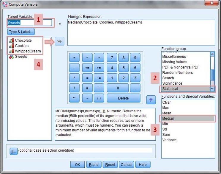
3.1. Computing Composite Scores
Compute composite scores by calculating the mean or median for each participant across the Likert-type items.
-
Access Compute Variable: Go to “Transform” -> “Compute Variable.”
-
Target Variable: Enter a name for the new composite variable (e.g., “OverallAttitude”).
-
Numeric Expression: Enter the formula to calculate the mean or median.
- Mean:
MEAN(Item1, Item2, Item3, Item4, Item5) - Median:
MEDIAN(Item1, Item2, Item3, Item4, Item5)
- Mean:
-
OK: Click “OK” to compute the new variable.
3.2. Descriptive Statistics and Visualization
Compute descriptive statistics (mean, median, standard deviation) for each group and visualize the data using histograms or box plots.
- Access Descriptive Statistics: Go to “Analyze” -> “Descriptive Statistics” -> “Descriptives.”
- Select Variables: Move the composite scores into the “Variables” box.
- Options: Click on “Options” and select the descriptive statistics you want to calculate (e.g., mean, standard deviation, minimum, maximum).
- Continue and OK: Click “Continue” and then “OK” to run the analysis.
3.2.1. Visualizing Data with Histograms
- Access Histogram: Go to “Graphs” -> “Legacy Dialogs” -> “Histogram.”
- Select Variable: Move the composite score variable into the “Variable” box.
- Display Normal Curve: Check the “Display normal curve” box to overlay a normal distribution curve on the histogram.
- OK: Click “OK” to generate the histogram.
3.2.2. Visualizing Data with Boxplots
- Access Boxplot: Go to “Graphs” -> “Legacy Dialogs” -> “Boxplot.”
- Simple Boxplot: Choose “Simple” and select “Summaries of separate variables.”
- Define: Move the composite score variable into the “Boxes Represent” box.
- OK: Click “OK” to generate the boxplot.
3.3. Independent Samples T-Test
If comparing two independent groups, conduct an independent samples t-test.
- Access Independent Samples T-Test: Go to “Analyze” -> “Compare Means” -> “Independent-Samples T Test.”
- Test Variable(s): Move the composite score variable into the “Test Variable(s)” box.
- Grouping Variable: Move the grouping variable (the variable that distinguishes the two groups) into the “Grouping Variable” box.
- Define Groups: Click on “Define Groups” and enter the values that represent the two groups (e.g., 1 and 2).
- Continue and OK: Click “Continue” and then “OK” to run the analysis.
3.4. Mann-Whitney U Test
For non-parametric comparison of two independent groups, use the Mann-Whitney U test.
- Access Mann-Whitney U Test: Go to “Analyze” -> “Nonparametric Tests” -> “Legacy Dialogs” -> “2 Independent Samples.”
- Test Variable(s): Move the composite score variable into the “Test Variable List” box.
- Grouping Variable: Move the grouping variable into the “Grouping Variable” box.
- Define Groups: Click on “Define Groups” and enter the values that represent the two groups.
- Test Type: Ensure “Mann-Whitney U” is checked.
- OK: Click “OK” to run the analysis.
3.5. Paired Samples T-Test
If comparing two related groups (e.g., pre-test and post-test scores), use a paired samples t-test.
- Access Paired-Samples T Test: Go to “Analyze” -> “Compare Means” -> “Paired-Samples T Test.”
- Select Variables: Select the two composite score variables you want to compare (e.g., “PreTestScore” and “PostTestScore”) and move them into the “Paired Variables” box.
- OK: Click “OK” to run the analysis.
3.6. Wilcoxon Signed-Rank Test
For non-parametric comparison of two related groups, use the Wilcoxon signed-rank test.
- Access Wilcoxon Signed-Rank Test: Go to “Analyze” -> “Nonparametric Tests” -> “Legacy Dialogs” -> “2 Related Samples.”
- Select Variables: Select the two composite score variables you want to compare and move them into the “Paired Variables” box.
- Test Type: Ensure “Wilcoxon” is checked.
- OK: Click “OK” to run the analysis.
3.7. Chi-Square Test
The Chi-Square test is used to determine if there is a significant association between two categorical variables. When analyzing Likert scale data, this test is appropriate if you want to examine the relationship between two Likert-type questions or between a Likert-type question and another categorical variable.
3.7.1. Steps to Perform Chi-Square Test
- Open SPSS: Launch SPSS and load your data file.
- Access Crosstabs: Go to “Analyze” -> “Descriptive Statistics” -> “Crosstabs.”
- Select Variables:
- Move one of the Likert scale variables to the “Row(s)” box.
- Move the other variable (either another Likert scale variable or a categorical variable) to the “Column(s)” box.
- Statistics: Click on the “Statistics” button and check the “Chi-square” box.
- Cells (Optional): If you want to see the expected counts, click on the “Cells” button and check “Expected” under the “Counts” section.
- Continue and OK: Click “Continue” and then “OK” to run the analysis.
3.7.2. Interpreting the Chi-Square Test Results
- Chi-Square Statistic: This is the value calculated by the test.
- Degrees of Freedom (df): This indicates the number of independent pieces of information used to calculate the statistic.
- p-value (Asymptotic Significance): This is the most important value to consider. If the p-value is less than or equal to your chosen significance level (commonly 0.05), you reject the null hypothesis and conclude that there is a significant association between the two variables.
- Expected Counts: These are the counts you would expect in each cell if there was no association between the variables. Large differences between the observed and expected counts suggest a significant association.
3.8. Correlation Analysis
Correlation analysis is used to determine the strength and direction of a linear relationship between two continuous variables. Although Likert scale data is ordinal, correlation analysis can still provide valuable insights, especially when treating the data as interval.
3.8.1. Steps to Perform Correlation Analysis
- Open SPSS: Launch SPSS and load your data file.
- Access Correlate: Go to “Analyze” -> “Correlate” -> “Bivariate.”
- Select Variables: Move the two Likert scale variables you want to analyze into the “Variables” box.
- Correlation Coefficients: Choose the appropriate correlation coefficient:
- Pearson: This is suitable if you assume your Likert scale data can be treated as interval and is normally distributed.
- Spearman: This is a non-parametric test that is appropriate for ordinal data or when the assumption of normality is violated.
- Test of Significance: Ensure that “Two-tailed” is selected unless you have a specific reason to use a one-tailed test.
- Options (Optional): Click on the “Options” button to request additional statistics such as means and standard deviations.
- OK: Click “OK” to run the analysis.
3.8.2. Interpreting the Correlation Analysis Results
- Correlation Coefficient (r or ρ): This value ranges from -1 to +1 and indicates the strength and direction of the relationship.
- A positive value indicates a positive relationship (as one variable increases, the other tends to increase).
- A negative value indicates a negative relationship (as one variable increases, the other tends to decrease).
- The absolute value of the coefficient indicates the strength of the relationship:
- 0.00-0.19: Very weak
- 0.20-0.39: Weak
- 0.40-0.59: Moderate
- 0.60-0.79: Strong
- 0.80-1.00: Very strong
- p-value (Sig. (2-tailed)): This indicates the statistical significance of the correlation. If the p-value is less than or equal to your chosen significance level (commonly 0.05), you reject the null hypothesis and conclude that there is a significant correlation between the two variables.
4. Interpreting the Results
4.1. Interpreting Descriptive Statistics
When interpreting descriptive statistics for Likert scale data, focus on the median and mode as measures of central tendency. The mean can be used cautiously if the data is approximately normally distributed. Standard deviation provides information about the variability of responses.
4.2. Interpreting T-Test and Mann-Whitney U Test
If the p-value is less than your chosen significance level (e.g., 0.05), there is a statistically significant difference between the two groups. Report the t-statistic, degrees of freedom, and p-value for the t-test. For the Mann-Whitney U test, report the U statistic and p-value.
4.3. Interpreting Paired Samples Tests
For paired samples t-tests and Wilcoxon signed-rank tests, a significant p-value indicates a statistically significant difference between the two related groups. Report the t-statistic, degrees of freedom, and p-value for the t-test. For the Wilcoxon test, report the test statistic and p-value.
4.4. Effect Size Measures
To quantify the practical significance of your findings, calculate effect size measures. For t-tests, Cohen’s d is commonly used. For non-parametric tests, you can use rank-biserial correlation.
4.5. Reporting the Results
In your research report, clearly describe the methods used to analyze the Likert scale data. Include the descriptive statistics, test statistics, p-values, and effect sizes. Provide a clear and concise interpretation of the findings in the context of your research question.
5. Advanced Techniques
5.1. Factor Analysis
Factor analysis is a statistical method used to reduce a large number of variables into a smaller number of factors. In the context of Likert scales, factor analysis can help identify underlying dimensions or constructs that the items are measuring. This is particularly useful when you have a large number of Likert-type questions and want to understand the main factors influencing responses.
5.1.1. Types of Factor Analysis
- Exploratory Factor Analysis (EFA):
- Purpose: To explore the underlying factor structure of a set of variables without prior assumptions.
- Use Case: When you are unsure of the number of factors or which variables load onto which factors.
- Confirmatory Factor Analysis (CFA):
- Purpose: To test a pre-specified factor structure.
- Use Case: When you have a hypothesis about the number of factors and which variables should load onto each factor, based on theory or prior research.
5.1.2. Steps to Perform Exploratory Factor Analysis (EFA) in SPSS
- Open SPSS: Launch SPSS and load your data file.
- Access Factor Analysis: Go to “Analyze” -> “Dimension Reduction” -> “Factor.”
- Select Variables: Move the Likert scale variables you want to analyze into the “Variables” box.
- Extraction:
- Method: Choose the extraction method (e.g., Principal Components, Maximum Likelihood). Principal Components is commonly used for EFA.
- Analyze: Select “Correlation matrix.”
- Display: Check “Unrotated factor solution” and “Scree plot.”
- Extract: Choose how to determine the number of factors:
- Based on Eigenvalue: Factors with eigenvalues greater than 1.
- Fixed number of factors: Specify the number of factors to extract.
- Rotation:
- Method: Choose a rotation method (e.g., Varimax, Promax). Varimax is a common orthogonal rotation that simplifies the factors. Promax is an oblique rotation that allows factors to be correlated.
- Display: Check “Rotated solution.”
- Options:
- Missing Values: Choose how to handle missing values (e.g., Exclude cases listwise).
- Coefficient display format: Check “Sorted by size” to make the factor loadings easier to interpret.
- OK: Click “OK” to run the analysis.
5.1.3. Interpreting EFA Results
- Kaiser-Meyer-Olkin (KMO) and Bartlett’s Test:
- KMO: Should be greater than 0.6 to indicate sampling adequacy.
- Bartlett’s Test: Should be significant (p < 0.05) to indicate that the correlation matrix is not an identity matrix.
- Total Variance Explained:
- Indicates the percentage of variance in the original variables that is explained by the extracted factors.
- Scree Plot:
- Helps determine the number of factors to retain by looking for the “elbow” in the plot.
- Factor Loadings:
- Indicate the correlation between each variable and each factor. Loadings greater than 0.4 are generally considered significant.
- Factor Interpretation:
- Examine the variables that load highly on each factor and interpret the meaning of the factor.
5.2. Regression Analysis
Regression analysis is a statistical method used to examine the relationship between a dependent variable and one or more independent variables. In the context of Likert scales, regression analysis can be used to predict an outcome variable based on responses to Likert-type questions.
5.2.1. Types of Regression Analysis
- Linear Regression:
- Purpose: To predict a continuous dependent variable from one or more continuous or categorical independent variables.
- Use Case: When you want to predict an outcome variable that is measured on a continuous scale.
- Logistic Regression:
- Purpose: To predict a binary or categorical dependent variable from one or more continuous or categorical independent variables.
- Use Case: When you want to predict an outcome variable that is categorical (e.g., pass/fail, agree/disagree).
5.2.2. Steps to Perform Linear Regression in SPSS
- Open SPSS: Launch SPSS and load your data file.
- Access Linear Regression: Go to “Analyze” -> “Regression” -> “Linear.”
- Select Variables:
- Move the dependent variable (the variable you want to predict) into the “Dependent” box.
- Move the Likert scale variables (or composite scores) you want to use as predictors into the “Independent(s)” box.
- Statistics:
- Click on the “Statistics” button and check the following:
- Estimates: To display regression coefficients.
- Confidence intervals: To display confidence intervals for the coefficients.
- Model fit: To display R-squared.
- Descriptives: To display means and standard deviations of the variables.
- Part and partial correlations: To display the unique contribution of each predictor.
- Collinearity diagnostics: To check for multicollinearity.
- Click on the “Statistics” button and check the following:
- Plots:
- Click on the “Plots” button and request the following plots to check assumptions:
- ZRESID vs. ZPRED: To check for linearity and homoscedasticity.
- Histogram of residuals: To check for normality.
- Normal P-P plot of residuals: To check for normality.
- Click on the “Plots” button and request the following plots to check assumptions:
- Options:
- Missing Values: Choose how to handle missing values (e.g., Exclude cases listwise).
- OK: Click “OK” to run the analysis.
5.2.3. Interpreting Linear Regression Results
- R-squared:
- Indicates the proportion of variance in the dependent variable that is explained by the independent variables.
- Regression Coefficients (B):
- Indicate the change in the dependent variable for a one-unit increase in the independent variable, holding all other variables constant.
- Standardized Coefficients (Beta):
- Indicate the relative importance of each independent variable in predicting the dependent variable.
- p-values (Sig.):
- Indicate the statistical significance of each predictor. A p-value less than 0.05 indicates that the predictor is significantly related to the dependent variable.
- Collinearity Diagnostics:
- Check the VIF (Variance Inflation Factor) values. VIF values greater than 5 or 10 indicate multicollinearity, which can affect the stability and interpretability of the regression coefficients.
6. Common Mistakes to Avoid
6.1. Treating Likert Data as Interval Data
Treating Likert scale data as interval data is a common mistake that can lead to incorrect statistical inferences. Remember that Likert scale data is ordinal, meaning the intervals between response options are not necessarily equal.
6.2. Ignoring Reverse-Scored Items
Failing to recode reverse-scored items can lead to inaccurate composite scores and misleading results. Always check and recode reverse-scored items before conducting any analysis.
6.3. Not Assessing Internal Consistency
Combining Likert items without assessing internal consistency can result in a scale that does not reliably measure the intended construct. Always calculate Cronbach’s alpha to ensure the scale is internally consistent.
6.4. Using Inappropriate Statistical Tests
Using statistical tests designed for interval or ratio data on Likert scale data can lead to incorrect conclusions. Choose non-parametric tests when comparing groups or use caution when interpreting results from parametric tests.
7. Conclusion
Comparing two Likert scales in SPSS involves careful preparation of data, appropriate selection of statistical methods, and thorough interpretation of results. By following the steps outlined in this guide and avoiding common mistakes, you can effectively analyze and interpret Likert scale data to gain valuable insights for your research. For further assistance and detailed comparisons, visit COMPARE.EDU.VN, where you can find comprehensive resources to aid your decision-making process.
Address: 333 Comparison Plaza, Choice City, CA 90210, United States
Whatsapp: +1 (626) 555-9090
Website: COMPARE.EDU.VN
Don’t let data analysis intimidate you. With the right approach, you can unlock valuable insights from your research. Visit COMPARE.EDU.VN today and discover how to make informed decisions based on thorough and reliable comparisons.
8. FAQ Section
8.1. Can I use a t-test to compare Likert scale data?
While Likert scale data is ordinal, some researchers treat it as interval data and use t-tests, especially when the sample size is large and the data is approximately normally distributed. However, it is generally more appropriate to use non-parametric tests like the Mann-Whitney U test or Wilcoxon signed-rank test.
8.2. What is Cronbach’s alpha, and why is it important?
Cronbach’s alpha is a measure of internal consistency reliability for a scale or test. It assesses the extent to which the items within a scale measure the same construct. A Cronbach’s alpha of 0.7 or higher generally indicates good internal consistency.
8.3. How do I handle missing data in Likert scales?
There are several ways to handle missing data, including:
- Listwise deletion: Exclude cases with any missing values.
- Pairwise deletion: Use only the available data for each analysis.
- Imputation: Replace missing values with estimated values (e.g., mean imputation, median imputation).
8.4. What if my data is not normally distributed?
If your data is not normally distributed, use non-parametric tests like the Mann-Whitney U test, Wilcoxon signed-rank test, or Kruskal-Wallis test. These tests do not assume normality.
8.5. How do I recode reverse-scored items in SPSS?
Go to “Transform” -> “Recode into Different Variables.” Enter the old and new values for the reverse-scored item and create a new variable with the recoded values.
8.6. What is the difference between mean and median, and which should I use?
The mean is the average of the values, while the median is the middle value. For Likert scale data, the median is often preferred because it is less sensitive to extreme values and better represents the central tendency of ordinal data.
8.7. How do I interpret the p-value in statistical tests?
The p-value indicates the probability of obtaining the observed results (or more extreme results) if the null hypothesis is true. A p-value less than your chosen significance level (e.g., 0.05) indicates that the results are statistically significant, and you reject the null hypothesis.
8.8. Can I combine Likert scale items into a single score?
Yes, you can combine Likert scale items into a single composite score by calculating the mean or median of the items, provided that the scale has good internal consistency (Cronbach’s alpha ≥ 0.7).
8.9. What are effect sizes, and why are they important?
Effect sizes are measures of the magnitude of an effect or relationship. They provide information about the practical significance of the findings beyond statistical significance. Common effect size measures include Cohen’s d for t-tests and rank-biserial correlation for non-parametric tests.
8.10. Where can I find more resources for analyzing Likert scale data?
You can find more resources and detailed comparisons at COMPARE.EDU.VN.
9. Additional Resources
9.1. Online Tutorials and Courses
- SPSS Tutorials: Numerous online tutorials are available that cover the basics of using SPSS for statistical analysis. Websites like LinkedIn Learning, Coursera, and YouTube offer comprehensive courses.
- Statistical Analysis Guides: Many universities and research institutions provide online guides on statistical analysis, including specific sections on Likert scale data.
9.2. Books
- Discovering Statistics Using IBM SPSS Statistics by Andy Field: A comprehensive guide to statistical analysis using SPSS, covering a wide range of topics and techniques.
- SPSS Survival Manual by Julie Pallant: A practical guide to using SPSS for data analysis, with step-by-step instructions and clear explanations.
9.3. Academic Journals and Articles
- Journal of Applied Measurement: Publishes articles on the theory and practice of measurement, including the use of Likert scales.
- Educational and Psychological Measurement: Features research on measurement and evaluation in education and psychology.
9.4. Conference Presentations and Workshops
- American Educational Research Association (AERA): Offers presentations and workshops on quantitative research methods, including the analysis of Likert scale data.
- American Psychological Association (APA): Provides resources and training on statistical analysis and research methodology.
By utilizing these resources and following the guidelines provided in this article, you can confidently analyze and interpret Likert scale data in SPSS to gain valuable insights for your research. Remember to visit compare.edu.vn for more comprehensive comparisons and assistance with your decision-making process.