Comparing two groups when you have multiple measurements per individual can be tricky, but it’s crucial for drawing accurate conclusions. This guide from COMPARE.EDU.VN offers clear methods to address this challenge, ensuring robust statistical analysis and reliable results. We’ll explore various statistical approaches, from t-tests to mixed-effects models, and delve into handling non-normal data and unequal group sizes. Understanding these techniques will empower you to make informed comparisons and avoid common pitfalls in data analysis. Discover the right way to analyze data with multiple measurements per subject, improve your understanding of statistical analysis, and implement best practices for comparing groups, helping you draw the most reliable conclusions.
1. Understanding the Challenge of Multiple Measurements
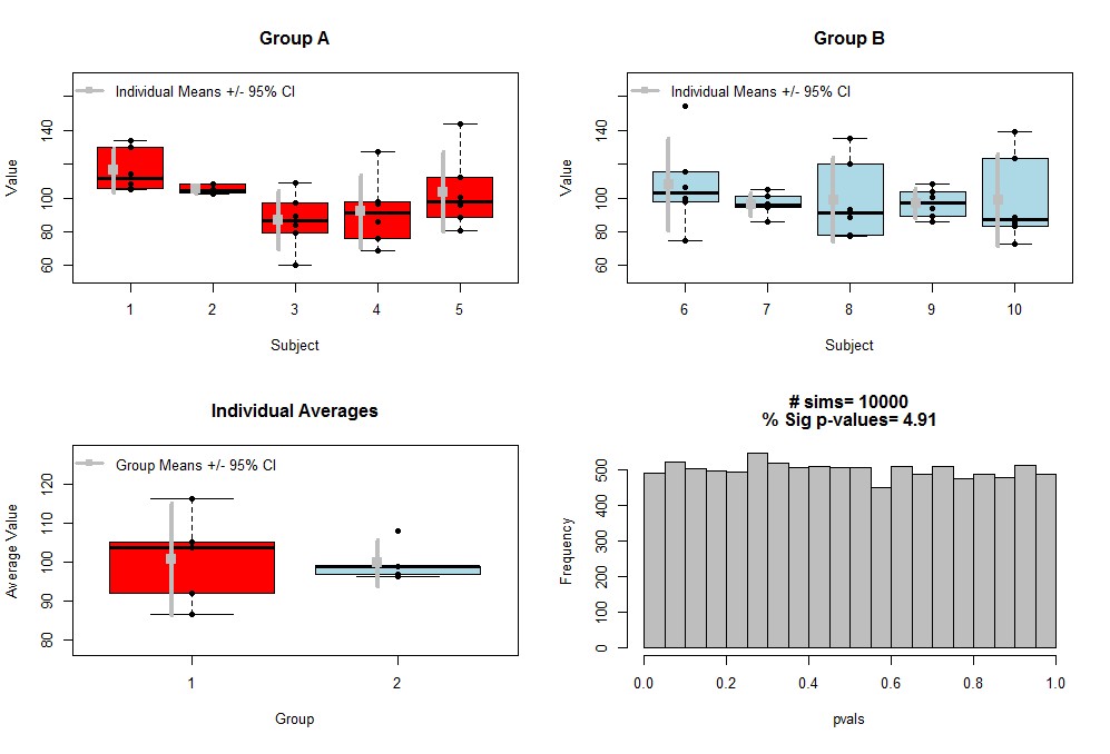
When dealing with multiple measurements within individuals across two groups (e.g., a treatment group and a control group), the key challenge is accounting for the within-subject variability. Simply averaging individual measurements and performing a standard t-test can underestimate the true variability, leading to inflated false-positive rates. This occurs because individual means are themselves estimates, and ignoring the within-subject variance can lead to overly precise, but potentially misleading, group comparisons.
To illustrate, imagine you are testing a new drug to lower blood pressure. You take six measurements from each of five patients in the treatment group and five in the control group. If you average each patient’s six readings and then compare the group averages with a t-test, you might find a significant difference. However, this approach fails to consider that some patients’ blood pressure varies more than others, which affects the reliability of each patient’s average.
1.1. Identifying Key Issues in Multiple Measurements
Before diving into analytical methods, it’s crucial to identify potential issues in your data:
- Within-Subject Variability: How much do measurements vary within the same individual? High variability can obscure true differences between groups.
- Correlation of Variance and Mean: Is the within-subject variance related to the mean? For instance, do individuals with higher mean values also have larger variances?
- Data Distribution: Are the measurements normally distributed? Non-normal data may require different analytical approaches.
- Floor or Ceiling Effects: Are there limitations on the range of possible values (e.g., a floor effect where many measurements are near zero)?
- Unequal Group Sizes: Do the groups have the same number of participants?
- Outliers: Are there extreme values that could disproportionately influence the results?
1.2. The Importance of Accounting for Within-Subject Variability
Failing to account for within-subject variability can lead to incorrect conclusions. Suppose you’re comparing two teaching methods by giving students multiple tests. If some students consistently perform differently on each test due to factors like test anxiety, simply averaging the scores would mask this variability. A proper analysis method would account for these individual differences to accurately compare the effectiveness of the teaching methods.
Understanding these nuances is essential for choosing the appropriate statistical method. COMPARE.EDU.VN provides tools and comparisons to help you assess these factors, ensuring you select the most accurate and reliable analysis technique for your specific dataset.
2. Choosing the Right Statistical Test
Selecting the appropriate statistical test depends on the nature of your data and the specific research question. Here are several options for comparing two groups with multiple measurements, each with its strengths and weaknesses.
2.1. Paired T-Test: When It’s Appropriate
A paired t-test is suitable when you have two measurements per subject and want to compare the means. This test is designed for scenarios where the measurements are naturally paired, such as pre- and post-treatment readings.
2.1.1. How the Paired T-Test Works
The paired t-test calculates the difference between each pair of measurements, then tests whether the mean of these differences is significantly different from zero. This accounts for the correlation between the paired measurements.
2.1.2. Example of Paired T-Test
Consider a study where you measure participants’ reaction times before and after consuming caffeine. You would use a paired t-test to determine if caffeine significantly changes reaction times, accounting for individual differences in baseline reaction times.
2.2. Repeated Measures ANOVA: Handling Multiple Time Points
Repeated Measures ANOVA (Analysis of Variance) is an extension of the paired t-test for situations where you have more than two measurements per subject.
2.2.1. Understanding Repeated Measures ANOVA
This method tests whether there are significant differences between the means of the repeated measurements while controlling for individual variability. It partitions the total variance into between-subject and within-subject components.
2.2.2. Practical Application of Repeated Measures ANOVA
Suppose you are tracking the performance of students on weekly quizzes over a semester. Repeated Measures ANOVA can help determine if there are significant changes in student performance over time, accounting for each student’s individual learning curve.
2.3. Linear Mixed-Effects Models: Flexibility and Power
Linear Mixed-Effects Models (LMEMs) are powerful and flexible tools for analyzing data with multiple measurements per subject, especially when dealing with complex data structures.
2.3.1. Core Concepts of Linear Mixed-Effects Models
LMEMs include both fixed effects (factors that you manipulate or measure) and random effects (factors that represent individual variability). This allows for modeling both the overall group differences and the individual deviations from those differences.
2.3.2. Benefits of Using Linear Mixed-Effects Models
- Handles Unequal Measurements: LMEMs can handle situations where subjects have different numbers of measurements.
- Accommodates Missing Data: They can accommodate missing data points without requiring complete datasets for each subject.
- Models Complex Dependencies: LMEMs can model complex dependencies between measurements, such as time-related trends.
- Accounts for Non-Independence: They correctly account for the non-independence of repeated measurements within subjects.
2.3.3. Real-World Example of Linear Mixed-Effects Models
Consider a clinical trial where patients receive a treatment, and their symptoms are assessed at multiple time points. LMEMs can model the effect of the treatment over time, accounting for individual patient responses and any missing data.
2.4. Generalized Estimating Equations: An Alternative Approach
Generalized Estimating Equations (GEEs) provide another approach for analyzing longitudinal or repeated measures data.
2.4.1. How Generalized Estimating Equations Work
GEEs model the marginal means while accounting for the correlation between repeated measurements within subjects. They are particularly useful when the normality assumption of LMEMs is violated.
2.4.2. Strengths and Weaknesses of Generalized Estimating Equations
- Robust to Non-Normality: GEEs are robust to non-normality, making them suitable for data that do not follow a normal distribution.
- Focus on Population-Level Effects: They focus on estimating the population-level effects, rather than individual-level effects.
- Requires Careful Specification of Correlation Structure: The correlation structure between repeated measurements must be carefully specified.
2.4.3. Example Use Case for Generalized Estimating Equations
In a study examining the effect of a new educational intervention on student test scores, GEEs can be used to model the average change in test scores across all students, accounting for the fact that each student’s scores are correlated over time.
2.5. Non-Parametric Tests: When Normality Is Not Assumed
When your data do not meet the assumptions of normality, non-parametric tests offer a robust alternative.
2.5.1. Wilcoxon Signed-Rank Test
The Wilcoxon Signed-Rank Test is the non-parametric equivalent of the paired t-test. It assesses whether the median difference between pairs of measurements is significantly different from zero.
2.5.2. Friedman Test
The Friedman Test is the non-parametric equivalent of the Repeated Measures ANOVA. It tests whether there are significant differences between the medians of the repeated measurements.
2.5.3. When to Use Non-Parametric Tests
Use non-parametric tests when your data are not normally distributed, or when you have ordinal data (e.g., rankings). These tests make fewer assumptions about the underlying distribution of the data.
2.6. Choosing the Best Test for Your Data
Selecting the most appropriate statistical test depends on several factors:
- Number of Measurements: Are there two measurements per subject (paired t-test, Wilcoxon Signed-Rank Test) or more than two (Repeated Measures ANOVA, Friedman Test, LMEMs, GEEs)?
- Data Distribution: Is the data normally distributed? If not, consider non-parametric tests or GEEs.
- Data Structure: Are there missing data points or unequal numbers of measurements per subject? LMEMs are well-suited for these situations.
- Research Question: Are you interested in individual-level effects (LMEMs) or population-level effects (GEEs)?
COMPARE.EDU.VN can guide you through these considerations, providing detailed comparisons of statistical tests to ensure you choose the method that best fits your data and research goals.
3. Implementing the Analysis
Once you’ve chosen the appropriate statistical test, the next step is to implement the analysis. This involves preparing your data, running the test using statistical software, and interpreting the results.
3.1. Data Preparation
Before running any statistical test, it’s essential to prepare your data properly. This includes:
- Cleaning the Data: Remove or correct any errors, inconsistencies, or outliers.
- Structuring the Data: Organize your data into a format suitable for the chosen statistical software. This usually involves creating a data frame or table with columns for subject IDs, group assignments, and measurements.
- Checking Assumptions: Verify that your data meet the assumptions of the chosen statistical test. For example, check for normality using histograms or normality tests.
3.2. Using Statistical Software (R, SPSS, etc.)
Statistical software packages like R, SPSS, and SAS provide tools for running the statistical tests discussed above.
3.2.1. R Examples
R is a powerful and flexible statistical programming language. Here are examples of how to implement some of the tests:
- Paired T-Test:
t.test(data$measurement1, data$measurement2, paired = TRUE)- Repeated Measures ANOVA:
library(ez) ezANOVA( data = data, dv = .(measurement), wid = .(subjectID), within = .(time), detailed = TRUE)- Linear Mixed-Effects Model:
library(lme4) model <- lmer(measurement ~ group * time + (1|subjectID), data = data) anova(model)- Generalized Estimating Equations:
library(geepack) model <- geeglm(measurement ~ group * time, id = subjectID, data = data, family = gaussian, corstr = "exchangeable") summary(model)3.2.2. SPSS Examples
SPSS is a user-friendly statistical software package with a graphical interface. Here are examples of how to implement some of the tests:
-
Paired T-Test:
- Go to Analyze > Compare Means > Paired-Samples T Test.
- Select the two measurement variables and click OK.
-
Repeated Measures ANOVA:
- Go to Analyze > General Linear Model > Repeated Measures.
- Define the within-subject factor (e.g., “time”) and specify the number of levels.
- Add the measurements to the within-subject variables and click OK.
-
Linear Mixed-Effects Model:
- Go to Analyze > Mixed Models > Linear.
- Specify the dependent variable (measurement), fixed factors (group, time), and random effects (subjectID).
- Click OK to run the model.
3.3. Interpreting the Results
Interpreting the results of your statistical test involves examining the p-value, effect size, and confidence intervals.
3.3.1. P-Value
The p-value indicates the probability of observing the data (or more extreme data) if there is no true difference between the groups. A p-value less than a predetermined significance level (usually 0.05) suggests that the difference is statistically significant.
3.3.2. Effect Size
The effect size quantifies the magnitude of the difference between the groups. Common effect size measures include Cohen’s d (for t-tests) and partial eta-squared (for ANOVA). A larger effect size indicates a more substantial difference.
3.3.3. Confidence Intervals
Confidence intervals provide a range of values within which the true population parameter is likely to fall. A 95% confidence interval means that if you were to repeat the study many times, 95% of the confidence intervals would contain the true population parameter.
3.4. Addressing Non-Normal Data
If your data are not normally distributed, you have several options:
- Transform the Data: Apply a mathematical transformation (e.g., log transformation, square root transformation) to make the data more normally distributed.
- Use Non-Parametric Tests: Choose non-parametric tests that do not assume normality.
- Use Robust Methods: Use robust statistical methods that are less sensitive to deviations from normality.
3.5. Handling Unequal Group Sizes
When the groups have unequal numbers of participants, it’s essential to use statistical methods that can handle this situation appropriately. LMEMs and GEEs are well-suited for analyzing data with unequal group sizes.
COMPARE.EDU.VN offers detailed guides and tutorials on using statistical software, interpreting results, and addressing common data issues. This ensures you can perform a robust and accurate analysis of your data.
4. Advanced Considerations and Techniques
Beyond the basic statistical tests, there are several advanced considerations and techniques that can further enhance your analysis.
4.1. Accounting for Covariates
Covariates are variables that may influence the outcome but are not the primary focus of your study. Including covariates in your analysis can help control for confounding factors and increase the precision of your results.
4.1.1. Incorporating Covariates in LMEMs
In LMEMs, covariates can be easily added as fixed effects in the model. This allows you to assess the effect of the primary factors of interest while controlling for the influence of the covariates.
4.1.2. Example of Covariate Adjustment
Suppose you are comparing the effectiveness of two weight loss programs, and you suspect that age and baseline weight may influence the outcome. You can include age and baseline weight as covariates in your LMEM to adjust for their effects.
4.2. Handling Missing Data
Missing data is a common problem in repeated measures studies. There are several approaches for handling missing data:
4.2.1. Complete Case Analysis
Complete case analysis involves excluding any subject with missing data. This approach is simple but can lead to biased results if the missing data are not missing completely at random (MCAR).
4.2.2. Imputation
Imputation involves filling in the missing data with estimated values. Common imputation methods include mean imputation, median imputation, and multiple imputation.
4.2.3. Model-Based Approaches
Model-based approaches, such as LMEMs, can handle missing data directly without requiring imputation. These models use all available data to estimate the parameters of interest.
4.3. Addressing Non-Linear Relationships
In some cases, the relationship between the variables may not be linear. In these situations, you may need to use non-linear models or transform the data to linearize the relationship.
4.3.1. Non-Linear Mixed-Effects Models
Non-linear mixed-effects models can be used to model non-linear relationships between the variables. These models are more complex but can provide a better fit to the data.
4.3.2. Transformation
Transforming the data can sometimes linearize the relationship between the variables. Common transformations include log transformation, square root transformation, and reciprocal transformation.
4.4. Reporting Your Results
When reporting your results, it’s essential to provide sufficient detail so that others can understand and replicate your analysis. This includes:
- Describing the Data: Provide descriptive statistics for each group, including means, standard deviations, and sample sizes.
- Describing the Statistical Methods: Clearly describe the statistical tests used, including any adjustments for covariates or missing data.
- Reporting the Results: Report the p-value, effect size, and confidence intervals for each test.
- Interpreting the Results: Interpret the results in the context of your research question.
COMPARE.EDU.VN offers resources and guidelines for reporting your results in a clear and comprehensive manner. This ensures that your findings are communicated effectively and can be easily understood by others.
5. Case Studies and Examples
To further illustrate the application of these methods, let’s consider several case studies and examples.
5.1. Clinical Trial: Comparing Drug Efficacy
In a clinical trial comparing the efficacy of two drugs for treating hypertension, patients are randomly assigned to either drug A or drug B. Blood pressure measurements are taken at baseline, and then weekly for eight weeks.
5.1.1. Data Analysis
An LMEM can be used to analyze the data, with drug group and time as fixed effects and patient ID as a random effect. Covariates such as age, sex, and baseline blood pressure can be included in the model to adjust for confounding factors.
5.1.2. Interpretation
The results of the LMEM can reveal whether there is a significant difference in blood pressure reduction between the two drugs over time, accounting for individual patient responses and any missing data.
5.2. Educational Study: Evaluating Teaching Methods
In an educational study evaluating the effectiveness of two teaching methods, students are randomly assigned to either method A or method B. Students’ performance is assessed using multiple quizzes throughout the semester.
5.2.1. Data Analysis
A GEE can be used to analyze the data, with teaching method and time as fixed effects and student ID as the subject variable. This approach is robust to non-normality and focuses on estimating the population-level effects.
5.2.2. Interpretation
The results of the GEE can indicate whether there is a significant difference in student performance between the two teaching methods, accounting for the correlation between repeated measurements within students.
5.3. Psychological Experiment: Measuring Cognitive Performance
In a psychological experiment measuring cognitive performance, participants complete a series of tasks at different levels of difficulty. Performance is measured by reaction time and accuracy.
5.3.1. Data Analysis
Repeated Measures ANOVA or LMEM can be used to analyze the data, with task difficulty as a within-subject factor and group (e.g., control vs. experimental) as a between-subject factor.
5.3.2. Interpretation
The results can reveal whether there is a significant interaction between task difficulty and group, indicating that the effect of task difficulty on cognitive performance differs between the two groups.
6. Best Practices for Comparing Groups with Multiple Measurements
To ensure the validity and reliability of your analysis, follow these best practices:
- Understand Your Data: Carefully examine your data to identify potential issues such as within-subject variability, non-normality, and missing data.
- Choose the Appropriate Statistical Test: Select the statistical test that best fits your data and research question. Consider factors such as the number of measurements, data distribution, and data structure.
- Prepare Your Data: Clean and structure your data properly before running any statistical test.
- Check Assumptions: Verify that your data meet the assumptions of the chosen statistical test.
- Use Statistical Software: Use statistical software packages like R, SPSS, or SAS to implement the analysis.
- Interpret the Results: Examine the p-value, effect size, and confidence intervals to interpret the results.
- Address Non-Normality: Use transformations, non-parametric tests, or robust methods to address non-normality.
- Handle Missing Data: Use appropriate methods for handling missing data, such as imputation or model-based approaches.
- Account for Covariates: Include covariates in your analysis to control for confounding factors.
- Report Your Results: Provide sufficient detail in your report so that others can understand and replicate your analysis.
COMPARE.EDU.VN is dedicated to providing you with the resources and tools you need to conduct rigorous and reliable statistical analyses. By following these best practices, you can ensure that your comparisons are accurate, meaningful, and contribute to a better understanding of your research area.
7. Common Pitfalls to Avoid
Analyzing data with multiple measurements can be complex, and there are several common pitfalls to avoid:
- Ignoring Within-Subject Variability: Failing to account for within-subject variability can lead to inflated false-positive rates.
- Assuming Normality: Assuming normality when the data are not normally distributed can lead to incorrect conclusions.
- Ignoring Missing Data: Ignoring missing data or using inappropriate methods for handling missing data can lead to biased results.
- Failing to Account for Covariates: Failing to account for covariates can lead to confounding and inaccurate conclusions.
- Over-Interpreting Results: Over-interpreting the results or drawing causal inferences without sufficient evidence can lead to misleading conclusions.
8. Resources and Tools on COMPARE.EDU.VN
COMPARE.EDU.VN offers a variety of resources and tools to help you compare groups with multiple measurements:
- Detailed Guides and Tutorials: Step-by-step guides and tutorials on how to implement various statistical tests using R, SPSS, and SAS.
- Statistical Test Comparisons: Detailed comparisons of statistical tests, including their strengths, weaknesses, and assumptions.
- Data Analysis Examples: Real-world examples of how to analyze data with multiple measurements using different statistical methods.
- Reporting Guidelines: Guidelines for reporting your results in a clear and comprehensive manner.
- Expert Support: Access to expert statisticians who can provide guidance and support for your data analysis.
9. Frequently Asked Questions (FAQ)
Q1: What is the main challenge when comparing two groups with multiple measurements?
The main challenge is accounting for within-subject variability to avoid inflated false-positive rates.
Q2: When should I use a paired t-test?
Use a paired t-test when you have two measurements per subject and want to compare the means, such as pre- and post-treatment readings.
Q3: What is Repeated Measures ANOVA and when is it appropriate?
Repeated Measures ANOVA is an extension of the paired t-test for situations where you have more than two measurements per subject, testing for significant differences between the means of the repeated measurements while controlling for individual variability.
Q4: What are Linear Mixed-Effects Models (LMEMs) and why are they useful?
LMEMs are powerful tools that include both fixed effects and random effects, allowing for modeling both the overall group differences and the individual deviations. They handle unequal measurements, accommodate missing data, model complex dependencies, and account for non-independence.
Q5: When should I consider using non-parametric tests?
Consider non-parametric tests when your data are not normally distributed, or when you have ordinal data, as these tests make fewer assumptions about the underlying distribution of the data.
Q6: How do I handle non-normal data in my analysis?
You can transform the data, use non-parametric tests, or use robust statistical methods that are less sensitive to deviations from normality.
Q7: What should I do if my groups have unequal numbers of participants?
Use statistical methods that can handle unequal group sizes appropriately, such as LMEMs and GEEs.
Q8: How can I account for covariates in my analysis?
Include covariates as fixed effects in LMEMs to adjust for their influence.
Q9: What are some common pitfalls to avoid when analyzing data with multiple measurements?
Common pitfalls include ignoring within-subject variability, assuming normality, ignoring missing data, failing to account for covariates, and over-interpreting results.
Q10: Where can I find resources and tools to help me compare groups with multiple measurements?
COMPARE.EDU.VN offers detailed guides, tutorials, statistical test comparisons, data analysis examples, reporting guidelines, and expert support.
10. Call to Action
Ready to make accurate and informed comparisons? Visit COMPARE.EDU.VN today to explore our comprehensive guides, tools, and resources. Whether you’re comparing clinical trial data, educational outcomes, or psychological experiments, we provide the expertise you need to confidently analyze your data and draw reliable conclusions. Our platform offers detailed comparisons of statistical tests, practical examples, and expert support to ensure you choose the right method for your research needs.
Address: 333 Comparison Plaza, Choice City, CA 90210, United States
Whatsapp: +1 (626) 555-9090
Website: COMPARE.EDU.VN
Don’t let complex data analysis hold you back. Let compare.edu.vn guide you to success!