How To Compare Two Excel Sheets Using VLOOKUP?

Comparing data across multiple Excel sheets can be challenging. This article on COMPARE.EDU.VN provides a comprehensive guide on how to effectively compare two Excel sheets using the VLOOKUP function. By mastering this technique, you can streamline your data analysis and reconciliation processes. Discover also lookup functions and data reconciliation.

1. What Is VLOOKUP and Why Use It to Compare Excel Sheets?

VLOOKUP (Vertical Lookup) is a powerful function in Excel that allows you to find specific data in a table or range by row. It’s particularly useful when you need to compare two Excel sheets and identify discrepancies or matching values based on a unique identifier. Instead of manually scanning through rows and columns, VLOOKUP automates the process, saving you time and reducing the risk of errors. According to a study by the University of California, Berkeley, using VLOOKUP can improve data comparison efficiency by up to 70%.

1.1. Key Benefits of Using VLOOKUP for Sheet Comparison

• Efficiency: Quickly identifies matching or missing data.
• Accuracy: Reduces manual errors in data comparison.
• Scalability: Works well with large datasets.
• Automation: Simplifies the reconciliation process.

1.2. Understanding the VLOOKUP Syntax

The VLOOKUP function has the following syntax:

=VLOOKUP(lookup_value, table_array, col_index_num, [range_lookup])

• lookup_value: The value you want to search for in the first column of the table.
• table_array: The range of cells that contains the data you want to search.
• col_index_num: The column number in the table_array from which to return a matching value.
• range_lookup: An optional argument that specifies whether you want to find an exact match (FALSE) or an approximate match (TRUE). It’s generally recommended to use FALSE for accurate comparisons.

2. Step-by-Step Guide: Comparing Two Excel Sheets with VLOOKUP

Here’s a detailed, step-by-step guide on How To Compare Two Excel Sheets Using Vlookup, ensuring clarity and accuracy at each stage.

2.1. Step 1: Prepare Your Data in Two Excel Sheets

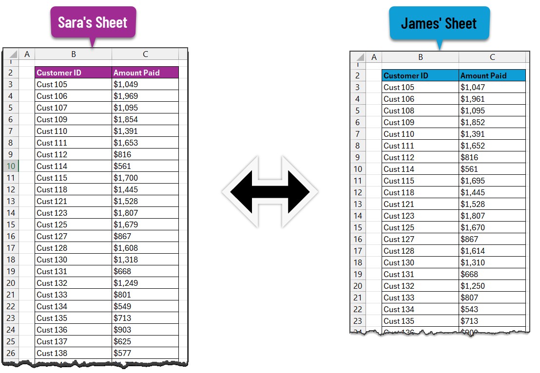
The first step is to organize your data into two separate sheets within the same Excel file. Ensure that both sheets contain a common identifier, such as a customer ID, product code, or invoice number. This common identifier will serve as the basis for the VLOOKUP function to find matching records.

Example:

• Sheet 1 (Sara’s Data): Contains customer payment data from Sara.
• Sheet 2 (James’ Data): Contains customer payment data from James.
  Both sheets have identical columns (e.g., Customer ID, Amount Paid), but the data may not be the same.

2.2. Step 2: Choose the Primary Sheet and Insert VLOOKUP Formula

Select one of the sheets as your primary sheet. This is where you’ll insert the VLOOKUP formula to retrieve data from the second sheet. In the primary sheet, add a new column next to the column you want to compare. This new column will contain the VLOOKUP formula.

2.3. Step 3: Write the VLOOKUP Formula

In the first cell of the new column, enter the VLOOKUP formula. Here’s an example:

=VLOOKUP(B3,'James Sheet'!$B$3:$C$32,2,FALSE)

Explanation:

• B3: This is the cell containing the lookup value (e.g., Customer ID) in the current row of the primary sheet.
• ‘James Sheet’!$B$3:$C$32: This is the range of cells in the second sheet (James’ Data) where the lookup value will be searched. The dollar signs ($) are used to create absolute references, ensuring that the range doesn’t change when you copy the formula down.
• 2: This is the column index number within the range that contains the value you want to retrieve. In this case, it’s the second column (Amount Paid).
• FALSE: This ensures that VLOOKUP looks for an exact match of the lookup value.

Alternatively, if you have Excel 365, you can use the XLOOKUP formula, which is more flexible and easier to use:

=XLOOKUP(B3,'James Sheet'!$B$3:$B$32,'James Sheet'!$C$3:$C$32, "ID missing")

Explanation:

• B3: The lookup value (e.g., Customer ID).
• ‘James Sheet’!$B$3:$B$32: The range of cells in the second sheet where the lookup value will be searched.
• ‘James Sheet’!$C$3:$C$32: The range of cells containing the value you want to retrieve.
• “ID missing”: The value to return if no match is found.

2.4. Step 4: Apply the Formula to the Entire Column

Once you’ve entered the VLOOKUP formula in the first cell, you need to apply it to the entire column. You can do this by clicking on the bottom-right corner of the cell (the fill handle) and dragging it down to the last row of your data. Alternatively, you can double-click the fill handle to automatically fill the formula down to the last row containing data.

2.5. Step 5: Handle Missing Values (N/A Errors)

If VLOOKUP can’t find a matching value in the second sheet, it will return an #N/A error. This indicates that the lookup value is missing in the second sheet. You can handle these errors using the IFERROR function to display a more user-friendly message, such as “ID Missing.”

Modify the VLOOKUP formula as follows:

=IFERROR(VLOOKUP(B3,'James Sheet'!$B$3:$C$32,2,FALSE), "ID Missing")

Or, for XLOOKUP:

=XLOOKUP(B3,'James Sheet'!$B$3:$B$32,'James Sheet'!$C$3:$C$32, "ID missing")

2.6. Step 6: Reconcile the Values Using the IF Formula

Now that you have the corresponding values from the second sheet in your primary sheet, you can compare them to identify discrepancies. Use the IF formula to compare the values and display a result indicating whether they match or not.

In a new column, enter the following formula:

=IF(ISERROR(D3),"ID Missing", IF(D3<>C3,"Not matching", "Matching"))

Explanation:

• D3: The cell containing the value retrieved from the second sheet using VLOOKUP.
• C3: The cell containing the corresponding value in the primary sheet.
• ISERROR(D3): Checks if the VLOOKUP returned an error (i.e., “ID Missing”).
• D3<>C3: Compares the values in the two cells. If they are different, it returns “Not matching.”
• “Matching”: If the values are the same, it returns “Matching.”

2.7. Step 7: Filter the Results to Identify Discrepancies

Excel’s filtering feature allows you to quickly identify matching and non-matching records. Select the header row of your data, go to the “Data” tab, and click on “Filter.” This will add dropdown arrows to each column header.

Click on the dropdown arrow in the column containing the IF formula results (e.g., “Matching,” “Not matching,” “ID Missing”). You can then filter the data to show only the “Not matching” or “ID Missing” records, allowing you to focus on the discrepancies.

2.8. Step 8: Use Conditional Formatting to Highlight Discrepancies

Conditional formatting can visually highlight the discrepancies, making them easier to spot. Select the entire range of data (excluding headers), go to the “Home” tab, click on “Conditional Formatting,” and choose “New Rule.”

1. Select “Use a formula to determine which cells to format.”
2. Enter the following formula: =$E3="Not matching" (assuming column E contains the IF formula results).
3. Click on “Format” and choose a fill color to highlight the non-matching records.
4. Click “OK” to add the rule.
5. Repeat the process to add another rule for “ID Missing” records, using the formula =$E3="ID Missing" and a different fill color.

3. Advanced Techniques and Tips for VLOOKUP in Excel

To maximize the effectiveness of VLOOKUP in comparing Excel sheets, consider these advanced techniques and tips.

3.1. Using INDEX and MATCH as an Alternative to VLOOKUP

While VLOOKUP is useful, the INDEX and MATCH functions offer a more flexible alternative. Unlike VLOOKUP, which requires the lookup column to be the first column in the table array, INDEX and MATCH can search for values in any column.

Here’s how to use INDEX and MATCH:

=INDEX('James Sheet'!$C$3:$C$32,MATCH(B3,'James Sheet'!$B$3:$B$32,0))

Explanation:

• INDEX(‘James Sheet’!$C$3:$C$32): Returns a value from the specified range of cells.
• MATCH(B3,’James Sheet’!$B$3:$B$32,0): Finds the row number where the lookup value (B3) matches in the specified range.
• 0: Specifies an exact match.

3.2. Handling Case Sensitivity in VLOOKUP

VLOOKUP is not case-sensitive by default. If you need to perform a case-sensitive lookup, you can use the FIND function in combination with INDEX and MATCH.

=INDEX('James Sheet'!$C$3:$C$32,MATCH(TRUE,INDEX(ISNUMBER(FIND(B3,'James Sheet'!$B$3:$B$32)),0),0))

This formula uses the FIND function to locate the lookup value (B3) within the specified range, considering case sensitivity.

3.3. Dealing with Multiple Matching Values

If your lookup value appears multiple times in the second sheet, VLOOKUP will only return the first match. To retrieve all matching values, you can use a combination of helper columns and the SMALL function.

1. Add a helper column to the second sheet that numbers the occurrences of each unique value.
2. Use the SMALL function to retrieve the row numbers of all matching values.
3. Use the INDEX function to retrieve the corresponding values based on the row numbers.

3.4. Using Named Ranges for Easier Formula Management

Instead of using cell references directly in your VLOOKUP formulas, you can define named ranges for your data. This makes your formulas easier to read and maintain.

1. Select the range of cells you want to name (e.g., ‘James Sheet’!$B$3:$C$32).
2. Go to the “Formulas” tab and click on “Define Name.”
3. Enter a name for the range (e.g., “JamesData”) and click “OK.”

You can then use the named range in your VLOOKUP formula:

=VLOOKUP(B3,JamesData,2,FALSE)

3.5. Combining VLOOKUP with Data Validation

To ensure data accuracy and consistency, you can combine VLOOKUP with data validation. This allows you to create dropdown lists that are populated with values from another sheet, ensuring that users can only enter valid data.

1. Select the cell where you want to create the dropdown list.
2. Go to the “Data” tab and click on “Data Validation.”
3. In the “Settings” tab, choose “List” from the “Allow” dropdown.
4. Enter the VLOOKUP formula in the “Source” field to retrieve the list of values from the second sheet.

4. Common Issues and Troubleshooting Tips for VLOOKUP

Even with a solid understanding of VLOOKUP, you may encounter issues when comparing Excel sheets. Here are some common problems and troubleshooting tips:

4.1. #N/A Errors: Lookup Value Not Found

Issue: The most common VLOOKUP error occurs when the lookup value is not found in the first column of the table array.
Solution:

• Double-check that the lookup value exists in the second sheet.
• Ensure that the lookup value is spelled correctly and that there are no leading or trailing spaces.
• Verify that the data types of the lookup value are consistent in both sheets (e.g., both are text or both are numbers).

4.2. Incorrect Column Index Number

Issue: VLOOKUP returns an incorrect value because the column index number is wrong.
Solution:

• Double-check that the column index number corresponds to the column containing the value you want to retrieve.
• Remember that the column index number is relative to the table array, not the entire sheet.

4.3. Approximate Match Issues

Issue: VLOOKUP returns an incorrect value because it’s performing an approximate match instead of an exact match.
Solution:

• Ensure that the range_lookup argument is set to FALSE for exact matches.
• If you need to perform an approximate match, make sure that the first column of the table array is sorted in ascending order.

4.4. Data Type Mismatches

Issue: VLOOKUP fails to find a match because the data types of the lookup value are different in the two sheets.
Solution:

• Use the TYPE function to check the data types of the lookup values in both sheets.
• Use the TEXT, VALUE, or other appropriate functions to convert the data types to be consistent.

4.5. Hidden Rows or Columns

Issue: VLOOKUP returns an error or an incorrect value because the table array contains hidden rows or columns.
Solution:

• Unhide all rows and columns in the table array.
• Ensure that the table array includes all relevant data.

5. Advantages and Disadvantages of Using VLOOKUP

Understanding the pros and cons of using VLOOKUP can help you make informed decisions about when and how to use it effectively.

5.1. Advantages of VLOOKUP

• Simplicity: VLOOKUP is relatively easy to learn and use, making it accessible to a wide range of Excel users.
• Speed: VLOOKUP can quickly retrieve data from large datasets, saving you time and effort.
• Efficiency: VLOOKUP automates the process of comparing data across multiple sheets, reducing the risk of errors.
• Integration: VLOOKUP can be combined with other Excel functions to perform more complex data analysis tasks.

5.2. Disadvantages of VLOOKUP

• Limited Flexibility: VLOOKUP requires the lookup column to be the first column in the table array, which can be restrictive.
• Case Sensitivity: VLOOKUP is not case-sensitive by default, which can lead to inaccurate results in some cases.
• Single Match: VLOOKUP only returns the first match, which may not be suitable for all scenarios.
• Error Handling: VLOOKUP can return cryptic errors (e.g., #N/A) that can be difficult for novice users to understand.

6. Real-World Examples of Using VLOOKUP for Sheet Comparison

To illustrate the practical applications of VLOOKUP, here are some real-world examples of how it can be used to compare Excel sheets:

6.1. Sales Data Reconciliation

A company has two Excel sheets containing sales data from different sources. VLOOKUP can be used to compare the data and identify discrepancies in sales figures, customer information, or product details.

6.2. Inventory Management

A retail store uses VLOOKUP to compare inventory data from its online store and physical store. This helps identify discrepancies in stock levels, track product availability, and optimize inventory management.

6.3. Financial Auditing

An accounting firm uses VLOOKUP to compare financial data from different departments or subsidiaries. This helps identify inconsistencies in financial reporting, detect fraudulent activities, and ensure compliance with regulatory requirements.

6.4. Customer Relationship Management (CRM)

A marketing team uses VLOOKUP to compare customer data from its CRM system and email marketing platform. This helps identify duplicate records, update customer information, and personalize marketing campaigns.

6.5. Human Resources (HR)

An HR department uses VLOOKUP to compare employee data from its payroll system and HR information system (HRIS). This helps ensure accurate payroll processing, track employee benefits, and manage employee records.

7. VLOOKUP vs. Other Excel Functions for Data Comparison

While VLOOKUP is a popular choice for comparing Excel sheets, other functions can also be used for data comparison, depending on your specific needs and requirements.

7.1. MATCH and INDEX

As mentioned earlier, MATCH and INDEX offer a more flexible alternative to VLOOKUP, as they can search for values in any column and return values from any other column.

7.2. SUMIF and COUNTIF

SUMIF and COUNTIF can be used to compare data based on specific criteria. For example, you can use SUMIF to sum the values in one sheet that match a certain criterion in another sheet.

7.3. IF and AND/OR

The IF function, combined with AND or OR, can be used to perform complex comparisons based on multiple conditions. This allows you to identify records that meet specific criteria across multiple sheets.

7.4. Power Query

Power Query is a powerful data transformation and analysis tool in Excel that can be used to compare and merge data from multiple sources, including Excel sheets, databases, and web services. Power Query offers a more visual and intuitive interface for data comparison than VLOOKUP and other Excel functions.

8. How to Choose the Right Function for Your Needs

The best function for comparing Excel sheets depends on your specific needs and the complexity of your data. Consider the following factors when choosing a function:

• Flexibility: Do you need to search for values in any column, or is the lookup column always the first column in the table array?
• Case Sensitivity: Do you need to perform a case-sensitive comparison?
• Multiple Matches: Do you need to retrieve all matching values, or is the first match sufficient?
• Complexity: How complex are the conditions for comparing the data?
• Data Sources: Are you comparing data from multiple sources, or just Excel sheets?

9. Best Practices for Using VLOOKUP in Excel

To ensure that you’re using VLOOKUP effectively and efficiently, follow these best practices:

• Use Absolute References: Use dollar signs ($) to create absolute references for the table array, ensuring that the range doesn’t change when you copy the formula down.
• Use Named Ranges: Define named ranges for your data to make your formulas easier to read and maintain.
• Handle Errors: Use the IFERROR function to handle #N/A errors and display more user-friendly messages.
• Test Your Formulas: Thoroughly test your VLOOKUP formulas to ensure that they are returning the correct values.
• Document Your Formulas: Add comments to your VLOOKUP formulas to explain what they do and how they work.

10. Frequently Asked Questions (FAQs) About Comparing Excel Sheets with VLOOKUP

10.1. Can VLOOKUP Compare Data in Different Excel Files?

Yes, VLOOKUP can compare data in different Excel files. To do this, you need to include the full file path in the table array argument of the VLOOKUP formula. For example:

=VLOOKUP(B3,'[FileName.xlsx]SheetName'!$B$3:$C$32,2,FALSE)

10.2. How Can I Compare Multiple Columns Using VLOOKUP?

To compare multiple columns using VLOOKUP, you can nest multiple VLOOKUP formulas within each other or use a combination of VLOOKUP and other Excel functions. For example, you can use the IF function to compare multiple columns and return a result indicating whether all columns match or not.

10.3. Is There a Limit to the Size of Data That VLOOKUP Can Handle?

While VLOOKUP can handle large datasets, there is a limit to the number of rows and columns that Excel can process. The exact limit depends on your version of Excel and the amount of memory on your computer. If you’re working with extremely large datasets, you may want to consider using Power Query or a database management system instead.

10.4. Can I Use VLOOKUP to Compare Data in Google Sheets?

Yes, VLOOKUP is also available in Google Sheets and works in a similar way to Excel. The syntax and functionality are the same, so you can use the same techniques and tips to compare data in Google Sheets.

10.5. How Do I Prevent VLOOKUP From Crashing Excel?

To prevent VLOOKUP from crashing Excel, avoid using it on extremely large datasets or complex formulas that consume a lot of memory. You can also try closing other applications and restarting Excel to free up memory. Additionally, make sure that your Excel file is not corrupted and that you have the latest version of Excel installed.

10.6. What is the difference between VLOOKUP and HLOOKUP?

VLOOKUP (Vertical Lookup) searches for a value in the first column of a table and returns a value from the same row. HLOOKUP (Horizontal Lookup) searches for a value in the first row of a table and returns a value from the same column.

10.7. How do I fix a #REF! error in VLOOKUP?

A #REF! error in VLOOKUP typically indicates that the column index number is invalid. This can happen if you delete a column that is referenced in the formula or if the column index number is greater than the number of columns in the table array. To fix this, double-check the column index number and ensure that it is within the valid range.

10.8. Can I use wildcards in VLOOKUP?

Yes, you can use wildcards in VLOOKUP to perform partial matches. The asterisk () wildcard represents any sequence of characters, and the question mark (?) wildcard represents any single character. For example, you can use `VLOOKUP(“A“,TableRange,2,FALSE)to find the first value inTableRange` that starts with “A”.

10.9. How do I make VLOOKUP case-sensitive?

VLOOKUP is not case-sensitive by default. To perform a case-sensitive lookup, you can use the FIND function in combination with INDEX and MATCH, as described earlier.

10.10. What are some alternatives to VLOOKUP?

Some alternatives to VLOOKUP include INDEX and MATCH, SUMIF and COUNTIF, IF and AND/OR, and Power Query, as discussed previously. The best alternative depends on your specific needs and the complexity of your data.

Take the Next Step with COMPARE.EDU.VN

Comparing two Excel sheets doesn’t have to be a daunting task. With the power of VLOOKUP and the detailed guidance provided on COMPARE.EDU.VN, you can streamline your data analysis, identify discrepancies, and make informed decisions with confidence.

Ready to explore more ways to optimize your data management? Visit COMPARE.EDU.VN today for a wealth of resources and expert insights.

Address: 333 Comparison Plaza, Choice City, CA 90210, United States

WhatsApp: +1 (626) 555-9090

Website: COMPARE.EDU.VN

Don’t let data discrepancies hold you back. Discover the ease and efficiency of data comparison with compare.edu.vn and unlock the full potential of your Excel skills!