How To Compare Two Excel Sheets For Matching Data?

Comparing two Excel sheets for matching data can be a daunting task, but COMPARE.EDU.VN provides a comprehensive guide to simplify the process. By employing methods like the MATCH function, conditional formatting, and other Excel functionalities, you can efficiently identify and highlight matching information, ensuring data accuracy and saving valuable time and effort. Let’s explore effective techniques for comparing Excel sheets and learn how to leverage comparison tools for optimal data analysis.

1. Why Is Comparing Two Excel Sheets For Matching Data Important?

Comparing two Excel sheets for matching data is crucial for data validation, error detection, and ensuring data integrity. This process helps in identifying discrepancies, inconsistencies, and duplicates, leading to more accurate and reliable data analysis. Whether you’re managing inventory, tracking sales, or analyzing financial data, knowing how to compare data efficiently in Excel is an invaluable skill.

1.1 Data Validation and Quality Control

Data validation is a critical process in data management that ensures the accuracy and reliability of data. By comparing two Excel sheets, you can identify any discrepancies and inconsistencies, ensuring that the data meets the required standards. According to a study by MIT, data quality issues cost businesses an average of 15% of their revenue. Using techniques like the MATCH function and conditional formatting can significantly reduce these errors and improve data quality.

1.2 Identifying Discrepancies and Errors

Excel is widely used for data entry, and human error is inevitable. Comparing two sheets helps in detecting these errors, such as incorrect entries, missing values, and typos. For example, if you are comparing sales data from two different periods, you can quickly identify any significant discrepancies that need further investigation. Tools like the IF function combined with the MATCH function can highlight these differences, allowing for prompt corrective actions.

1.3 Ensuring Data Integrity

Data integrity refers to the accuracy and consistency of data over its entire lifecycle. By regularly comparing Excel sheets, you can ensure that the data remains consistent and reliable. This is particularly important in industries such as finance and healthcare, where data integrity is paramount. Regular comparisons can prevent data corruption, unauthorized changes, and other issues that could compromise the integrity of your data.

1.4 Efficient Data Analysis

Comparing Excel sheets allows for more efficient data analysis by providing a clear view of the similarities and differences between datasets. This can help in identifying trends, patterns, and insights that would otherwise be difficult to spot. For example, by comparing customer data from two different marketing campaigns, you can determine which campaign was more successful in attracting and retaining customers.

1.5 Saving Time and Effort

Manually comparing two large Excel sheets can be time-consuming and tedious. By using Excel’s built-in functions and features, you can automate the comparison process and save valuable time and effort. Tools like the VLOOKUP and INDEX-MATCH functions can quickly find and match data, reducing the need for manual inspection.

2. What Are The Essential Excel Functions For Comparing Data?

Several Excel functions are essential for comparing data, including MATCH, VLOOKUP, INDEX-MATCH, and Conditional Formatting. Each function offers unique capabilities for identifying matching and differing data, making data comparison more efficient and accurate. Mastering these functions is key to effective data analysis in Excel.

2.1 The MATCH Function

The MATCH function is a powerful tool for finding the position of a specific value within a range of cells. It returns the relative position of an item in an array that matches a specified value in a specified order.

Syntax: =MATCH(lookup_value, lookup_array, [match_type])

lookup_value: The value you want to find.
lookup_array: The range of cells being searched.
match_type: Optional. Specifies how Excel matches the lookup_value with values in the lookup_array. Common values are 0 (exact match), 1 (less than), and -1 (greater than).

For example, to find the position of “Apple” in the range A1:A10, you would use the formula: =MATCH("Apple", A1:A10, 0).

2.2 The VLOOKUP Function

VLOOKUP (Vertical Lookup) is used to find a value in the first column of a range and return a value from a cell in the same row of a specified column. It is useful for pulling data from one sheet to another based on a common identifier.

Syntax: =VLOOKUP(lookup_value, table_array, col_index_num, [range_lookup])

lookup_value: The value you want to find.
table_array: The range of cells in which to search.
col_index_num: The column number in the table_array from which to return the matching value.
range_lookup: Optional. Specifies whether to find an exact or approximate match. TRUE for approximate, FALSE for exact.

For example, to find the price of “Apple” from a table in the range A1:B10 where the prices are in column B, you would use the formula: =VLOOKUP("Apple", A1:B10, 2, FALSE).

2.3 The INDEX-MATCH Function Combination

The INDEX-MATCH combination is a more flexible alternative to VLOOKUP. It allows you to look up values in a table based on both row and column criteria. INDEX returns the value of a cell in a table based on the row and column numbers, while MATCH finds the row or column number.

Syntax: =INDEX(array, row_num, [column_num]) and =MATCH(lookup_value, lookup_array, [match_type])

Combining them: =INDEX(return_array, MATCH(lookup_value, lookup_array, 0))

array: The range of cells from which to return a value.
row_num: The row number in the array from which to return a value.
column_num: Optional. The column number in the array from which to return a value.
lookup_value: The value you want to find.
lookup_array: The range of cells being searched.

For example, to find the price of “Apple” in the range B1:B10 using the names in A1:A10, you would use the formula: =INDEX(B1:B10, MATCH("Apple", A1:A10, 0)).

2.4 Conditional Formatting

Conditional Formatting allows you to highlight cells based on certain criteria. It’s useful for visually identifying matching or differing data in two sheets. You can create rules to highlight duplicate values, unique values, or values that meet specific conditions.

Steps to use Conditional Formatting:

Select the range of cells you want to format.
Go to Home > Conditional Formatting.
Choose a rule, such as Highlight Cells Rules > Duplicate Values.
Select the formatting you want to apply and click OK.

For example, to highlight duplicate values in a column, select the column, go to Conditional Formatting, choose “Highlight Cells Rules,” then “Duplicate Values,” and select a color to highlight the duplicates.

2.5 The IF Function

The IF function checks whether a condition is met and returns one value if true and another value if false. It can be used to compare values in two sheets and return a specific result based on whether the values match or differ.

Syntax: =IF(logical_test, value_if_true, value_if_false)

logical_test: The condition you want to evaluate.
value_if_true: The value to return if the condition is true.
value_if_false: The value to return if the condition is false.

For example, to compare the values in cell A1 of Sheet1 and cell A1 of Sheet2, you would use the formula: =IF(Sheet1!A1=Sheet2!A1, "Match", "No Match").

3. How Can You Compare Two Excel Sheets For Matching Data Using The Match Function?

Comparing two Excel sheets for matching data using the MATCH function involves identifying the position of a specific value in one sheet within a range in another sheet. This method helps in quickly locating matches and identifying missing entries. By combining MATCH with other functions like IF and ISNA, you can create powerful formulas for data comparison.

3.1 Preparing Your Worksheets

Before you start comparing data, ensure that your two worksheets are properly prepared. This includes organizing the data in a consistent format and ensuring that the columns you want to compare have similar data types.

Steps to Prepare Your Worksheets:

Open both Excel sheets in the same workbook.
Check for consistency in data types (e.g., numbers, text, dates).
Ensure that the columns you want to compare have similar headings and formats.
Remove any unnecessary rows or columns that might interfere with the comparison.

3.2 Using the MATCH Function to Find Matches

The MATCH function can be used to find the position of a value in one sheet within a range in another sheet. This is useful for identifying whether a specific value exists in both sheets.

Formula: =MATCH(lookup_value, lookup_array, [match_type])

Example:

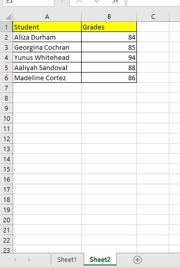
Suppose you have two sheets, “Sheet1” and “Sheet2,” and you want to check if the values in column A of Sheet2 exist in column A of Sheet1.

In Sheet2, select an empty column (e.g., column B).
Enter the following formula in cell B2: =MATCH(A2, Sheet1!A:A, 0)
Drag the formula down to apply it to all the rows in column A of Sheet2.

The formula returns the row number in Sheet1 where the value from Sheet2 is found. If the value is not found, the formula returns an error (#N/A).

3.3 Handling Errors with ISNA and IF Functions

When the MATCH function does not find a match, it returns an error (#N/A). To handle these errors and provide more informative results, you can combine the MATCH function with the ISNA and IF functions.

Formula: =IF(ISNA(MATCH(lookup_value, lookup_array, 0)), "Not Found", "Found")

Example:

Using the same scenario as above, you can modify the formula in Sheet2, column B to display “Found” if the value exists in Sheet1 and “Not Found” if it doesn’t.

In Sheet2, select column B.
Enter the following formula in cell B2: =IF(ISNA(MATCH(A2, Sheet1!A:A, 0)), "Not Found", "Found")
Drag the formula down to apply it to all the rows in column A of Sheet2.

This formula checks if the MATCH function returns an error (#N/A). If it does, the IF function displays “Not Found”; otherwise, it displays “Found.”

3.4 Highlighting Matching Data with Conditional Formatting

Conditional formatting can be used to visually highlight matching data in the two sheets. This makes it easier to quickly identify which values are present in both sheets.

Steps to Highlight Matching Data:

Select the data range in Sheet2 (e.g., column A).
Go to Home > Conditional Formatting > New Rule.
Select “Use a formula to determine which cells to format.”
Enter the following formula: =NOT(ISNA(MATCH(A2, Sheet1!A:A, 0)))
Click on Format to choose a formatting style (e.g., fill color).
Click OK to apply the formatting.

This conditional formatting rule highlights the cells in Sheet2 that have matching values in Sheet1.

3.5 Comparing Multiple Columns

You can extend the use of the MATCH function to compare multiple columns by combining it with other logical functions such as AND and OR.

Example:

Suppose you want to compare columns A and B in Sheet1 with columns C and D in Sheet2, and you want to find rows where both columns match.

In Sheet2, select an empty column (e.g., column E).
Enter the following formula in cell E2: =IF(AND(NOT(ISNA(MATCH(C2, Sheet1!A:A, 0))), NOT(ISNA(MATCH(D2, Sheet1!B:B, 0)))), "Match", "No Match")
Drag the formula down to apply it to all the rows in Sheet2.

This formula checks if both column C and column D in Sheet2 have matching values in columns A and B of Sheet1. If both columns match, the formula displays “Match”; otherwise, it displays “No Match.”

4. How To Highlight Matched Data Using Conditional Formatting?

Highlighting matched data using conditional formatting allows for a visual representation of similarities between two Excel sheets. This technique involves setting rules that automatically format cells based on whether they match corresponding cells in another sheet. This method is particularly useful for quickly identifying common entries and discrepancies.

4.1 Setting Up Conditional Formatting Rules

Conditional formatting rules are the foundation for highlighting matched data. These rules define the conditions under which cells will be formatted, such as when a cell’s value matches a value in another sheet.

Steps to Set Up Conditional Formatting Rules:

Select the range of cells in the first sheet that you want to format.
Go to Home > Conditional Formatting > New Rule.
In the “New Formatting Rule” dialog box, select “Use a formula to determine which cells to format.”
Enter the formula that defines the matching condition.
Click on Format to choose the formatting style (e.g., fill color, font color).
Click OK to apply the rule.

4.2 Using Formulas to Define Matching Conditions

Formulas are used to define the conditions under which cells will be formatted. These formulas typically involve comparing the values in the selected range with values in another sheet.

Common Formulas for Matching Conditions:

Exact Match: =A1=Sheet2!A1 (This formula checks if the value in cell A1 of the current sheet matches the value in cell A1 of Sheet2.)
Match with MATCH Function: =NOT(ISNA(MATCH(A1, Sheet2!A:A, 0))) (This formula checks if the value in cell A1 of the current sheet exists in column A of Sheet2.)

Example:

To highlight cells in Sheet1 that have the same value as the corresponding cells in Sheet2, follow these steps:

Select the range of cells in Sheet1 (e.g., A1:A10).
Go to Home > Conditional Formatting > New Rule.
Select “Use a formula to determine which cells to format.”
Enter the formula: =A1=Sheet2!A1
Click on Format to choose a fill color (e.g., green).
Click OK to apply the rule.

4.3 Applying Conditional Formatting Across Multiple Columns

Conditional formatting can be applied across multiple columns to highlight matching data in multiple sets of data. This involves adjusting the formulas to account for the different columns being compared.

Steps to Apply Conditional Formatting Across Multiple Columns:

Select the entire range of cells you want to format (e.g., A1:C10).
Go to Home > Conditional Formatting > New Rule.
Select “Use a formula to determine which cells to format.”
Enter the formula that defines the matching condition, adjusting the cell references as needed.
Click on Format to choose the formatting style.
Click OK to apply the rule.

Example:

To highlight rows in Sheet1 where both column A and column B match the corresponding values in Sheet2, use the following formula:

=AND(A1=Sheet2!A1, B1=Sheet2!B1)

4.4 Using Conditional Formatting to Identify Differences

Conditional formatting can also be used to identify differences between two sheets. This involves setting rules that highlight cells when their values do not match the corresponding values in another sheet.

Formula for Identifying Differences:

=A1<>Sheet2!A1 (This formula checks if the value in cell A1 of the current sheet is different from the value in cell A1 of Sheet2.)

Example:

To highlight cells in Sheet1 that have different values from the corresponding cells in Sheet2, follow these steps:

Select the range of cells in Sheet1 (e.g., A1:A10).
Go to Home > Conditional Formatting > New Rule.
Select “Use a formula to determine which cells to format.”
Enter the formula: =A1<>Sheet2!A1
Click on Format to choose a fill color (e.g., red).
Click OK to apply the rule.

4.5 Clearing Conditional Formatting Rules

If you need to remove or modify the conditional formatting rules, you can easily clear them from the selected range of cells.

Steps to Clear Conditional Formatting Rules:

Select the range of cells from which you want to clear the formatting.
Go to Home > Conditional Formatting > Clear Rules.
Choose “Clear Rules from Selected Cells” or “Clear Rules from Entire Sheet” as needed.

5. What Are The Advantages Of Using Index-Match Over Vlookup For Data Comparison?

While both INDEX-MATCH and VLOOKUP are used for data comparison and retrieval, INDEX-MATCH offers several advantages, including greater flexibility, the ability to look up values to the left, and improved performance with large datasets. Understanding these advantages can help you choose the best method for your data analysis needs.

5.1 Flexibility in Lookup Direction

One of the primary advantages of INDEX-MATCH over VLOOKUP is its flexibility in lookup direction. VLOOKUP can only search for a value in the first column of a range and return a value from a column to the right. INDEX-MATCH can look up values in any column and return values from any other column, regardless of their position.

Example:

Suppose you have a table with employee names in column B and their corresponding salaries in column A. With VLOOKUP, you would need to rearrange the columns to have the employee names in the first column. With INDEX-MATCH, you can easily find the salary of an employee using the following formula:

=INDEX(A:A, MATCH("Employee Name", B:B, 0))

5.2 Handling Inserted or Deleted Columns

INDEX-MATCH is more robust when dealing with inserted or deleted columns. VLOOKUP relies on a fixed column index number, which can break if columns are inserted or deleted. INDEX-MATCH, on the other hand, uses the column letter or name, which remains constant even if columns are added or removed.

Example:

If you have a VLOOKUP formula that retrieves data from the third column and you insert a new column, the VLOOKUP formula will now retrieve data from the fourth column, leading to incorrect results. INDEX-MATCH avoids this issue because it references the column directly.

5.3 Improved Performance with Large Datasets

INDEX-MATCH generally performs better than VLOOKUP with large datasets. VLOOKUP searches the entire table array, which can be slow with large datasets. INDEX-MATCH, on the other hand, uses the MATCH function to find the exact row number and then retrieves the value using INDEX, which is more efficient.

According to a study by Microsoft, INDEX-MATCH can be up to 50% faster than VLOOKUP when working with very large datasets.

5.4 More Readable and Maintainable Formulas

INDEX-MATCH formulas are often more readable and easier to maintain than VLOOKUP formulas. The INDEX and MATCH functions are separate and clearly define the lookup and return ranges, making the formula easier to understand and modify.

Example:

Consider the following VLOOKUP formula:

=VLOOKUP("Employee Name", A1:C100, 3, FALSE)

This formula is less clear than the equivalent INDEX-MATCH formula:

=INDEX(C1:C100, MATCH("Employee Name", A1:A100, 0))

The INDEX-MATCH formula clearly separates the return range (C1:C100) from the lookup range (A1:A100), making it easier to understand and modify.

5.5 Ability to Perform Two-Way Lookups

INDEX-MATCH can be easily extended to perform two-way lookups, where you look up values based on both row and column criteria. This is more complex to achieve with VLOOKUP.

Example:

Suppose you have a table with sales data for different products in rows and different months in columns. To find the sales for a specific product in a specific month, you can use the following INDEX-MATCH formula:

=INDEX(data_range, MATCH("Product Name", product_range, 0), MATCH("Month", month_range, 0))

6. How Can The If Function Be Used For Comparing Data In Excel?

The IF function is a versatile tool for comparing data in Excel, allowing you to perform conditional checks and return different values based on whether a condition is true or false. This function is particularly useful for identifying matches, differences, and specific criteria in your data.

6.1 Basic Syntax and Usage of the IF Function

The IF function evaluates a logical test and returns one value if the test is true and another value if the test is false.

Syntax: =IF(logical_test, value_if_true, value_if_false)

logical_test: The condition you want to evaluate.
value_if_true: The value to return if the condition is true.
value_if_false: The value to return if the condition is false.

Example:

To check if the value in cell A1 is greater than 10, you can use the following formula:

=IF(A1>10, "Greater than 10", "Less than or equal to 10")

6.2 Comparing Values in Two Sheets Using the IF Function

The IF function can be used to compare values in two different sheets and return a specific result based on whether the values match or differ.

Example:

To compare the values in cell A1 of Sheet1 and cell A1 of Sheet2, you can use the following formula in Sheet1:

=IF(A1=Sheet2!A1, "Match", "No Match")

This formula checks if the value in A1 of Sheet1 is equal to the value in A1 of Sheet2. If they are equal, the formula returns “Match”; otherwise, it returns “No Match.”

6.3 Using Nested IF Functions for Multiple Conditions

Nested IF functions allow you to check multiple conditions and return different values based on the outcome of each condition.

Example:

Suppose you want to compare the values in cell A1 of Sheet1 and cell A1 of Sheet2 and return different messages based on whether A1 is greater than, less than, or equal to the value in Sheet2!A1. You can use the following nested IF formula:

=IF(A1>Sheet2!A1, "Greater", IF(A1<Sheet2!A1, "Less", "Equal"))

This formula first checks if A1 is greater than Sheet2!A1. If it is, the formula returns “Greater.” If not, it checks if A1 is less than Sheet2!A1. If it is, the formula returns “Less.” If neither condition is true, the formula returns “Equal,” indicating that the values are the same.

6.4 Combining IF with Other Functions for Advanced Comparisons

The IF function can be combined with other functions like AND, OR, and NOT to create more complex comparison formulas.

Example:

Suppose you want to check if both the values in cell A1 and B1 of Sheet1 are equal to the values in cell A1 and B1 of Sheet2. You can use the following formula:

=IF(AND(A1=Sheet2!A1, B1=Sheet2!B1), "Both Match", "At Least One Does Not Match")

This formula uses the AND function to check if both conditions (A1=Sheet2!A1 and B1=Sheet2!B1) are true. If both conditions are true, the formula returns “Both Match”; otherwise, it returns “At Least One Does Not Match.”

6.5 Using IF to Identify Missing Data

The IF function can also be used to identify missing data in two sheets. For example, you can check if a value exists in one sheet but not in another.

Example:

Suppose you want to check if the values in column A of Sheet2 exist in column A of Sheet1. You can use the MATCH function in combination with the IF and ISNA functions to achieve this.

In Sheet2, select an empty column (e.g., column B).
Enter the following formula in cell B2: =IF(ISNA(MATCH(A2, Sheet1!A:A, 0)), "Not Found", "Found")
Drag the formula down to apply it to all the rows in column A of Sheet2.

This formula checks if the MATCH function returns an error (#N/A). If it does, the IF function displays “Not Found”; otherwise, it displays “Found.”

7. What Are Some Common Scenarios Where Comparing Excel Sheets Is Useful?

Comparing Excel sheets is useful in various scenarios, including data validation, reconciliation, duplicate detection, and data migration. Each scenario benefits from the ability to quickly and accurately identify similarities and differences between datasets.

7.1 Data Validation and Quality Assurance

Data validation is the process of ensuring that data is accurate, complete, and consistent. Comparing Excel sheets is a common method for validating data, especially when data is entered manually or imported from different sources.

Scenario:

A company collects customer data through an online form and a paper-based survey. To ensure the accuracy of the combined dataset, the data entry team compares the two Excel sheets containing the data from each source.

Benefits:

Identifies discrepancies in customer information (e.g., different addresses, phone numbers).
Ensures that all required fields are completed for each customer.
Reduces the risk of errors in marketing campaigns and customer communications.

7.2 Financial Reconciliation

Financial reconciliation involves comparing two sets of financial records to ensure that they match. This is a critical process for maintaining accurate financial statements and detecting fraud.

Scenario:

An accounting department compares the general ledger with bank statements to reconcile cash balances.

Benefits:

Identifies any unauthorized transactions or errors in the ledger.
Ensures that all deposits and withdrawals are accurately recorded.
Provides a clear audit trail for financial transactions.

7.3 Duplicate Data Detection

Duplicate data can lead to inaccurate reporting, wasted resources, and compliance issues. Comparing Excel sheets is an effective way to identify and remove duplicate entries.

Scenario:

A marketing team merges two customer lists from different marketing campaigns and needs to identify and remove duplicate contacts.

Benefits:

Reduces the cost of marketing campaigns by avoiding sending duplicate messages to the same customers.
Improves the accuracy of customer analytics and reporting.
Ensures compliance with data privacy regulations.

7.4 Data Migration

Data migration involves transferring data from one system to another. Comparing Excel sheets is essential for verifying that the data is accurately transferred and that no data is lost during the migration process.

Scenario:

A company migrates its customer database from an old CRM system to a new one. The data migration team compares the data in the old and new systems to ensure that all customer records are transferred correctly.

Benefits:

Ensures that all customer data is accurately transferred to the new system.
Reduces the risk of data loss or corruption during the migration process.
Minimizes disruptions to business operations.

7.5 Inventory Management

Accurate inventory management is essential for maintaining optimal stock levels and avoiding stockouts or excess inventory. Comparing Excel sheets is used to reconcile inventory records and identify discrepancies.

Scenario:

A retail company compares its physical inventory count with its inventory management system to identify any discrepancies.

Benefits:

Identifies any missing or misplaced inventory items.
Ensures that inventory records are accurate and up-to-date.
Reduces the risk of stockouts and lost sales.

8. What Are Some Tips For Efficiently Comparing Large Excel Sheets?

Comparing large Excel sheets can be challenging, but several tips can help you streamline the process, including sorting data, using filters, employing Excel tables, and leveraging external tools. These strategies can significantly improve efficiency and accuracy when dealing with extensive datasets.

8.1 Sorting Data for Easier Comparison

Sorting data can make it easier to identify matching and differing values by arranging the data in a logical order.

Steps to Sort Data:

Select the range of cells you want to sort.
Go to Data > Sort.
Choose the column you want to sort by and the sort order (e.g., ascending or descending).
Click OK to apply the sorting.

Example:

To compare customer names in two sheets, sort both sheets alphabetically by the customer name column. This makes it easier to visually identify matching names and any discrepancies.

8.2 Using Filters to Focus on Specific Data

Filters allow you to display only the rows that meet certain criteria, making it easier to focus on specific subsets of data.

Steps to Use Filters:

Select the range of cells you want to filter.
Go to Data > Filter.
Click the dropdown arrow in the column header to open the filter menu.
Choose the filter criteria you want to apply (e.g., specific values, date ranges).
Click OK to apply the filter.

Example:

To compare sales data for a specific product, filter both sheets to show only the rows that pertain to that product. This allows you to focus on the sales performance of that product across the two datasets.

8.3 Converting Data to Excel Tables

Excel tables provide several benefits for data comparison, including automatic column referencing and structured formulas.

Steps to Convert Data to an Excel Table:

Select the range of cells you want to convert to a table.
Go to Insert > Table.
Ensure that the “My table has headers” checkbox is selected if your data includes column headers.
Click OK to create the table.

Example:

Converting your data to Excel tables allows you to use structured formulas that automatically adjust when you add or remove rows and columns. This makes it easier to compare data across the two tables.

8.4 Using Excel’s “View Side by Side” Feature

Excel’s “View Side by Side” feature allows you to display two sheets or workbooks next to each other, making it easier to visually compare the data.

Steps to Use “View Side by Side”:

Open both Excel sheets or workbooks you want to compare.
Go to View > View Side by Side.
If you have multiple workbooks open, select the workbook you want to compare with the current one.
Enable “Synchronous Scrolling” to scroll both sheets simultaneously.

8.5 Leveraging External Tools and Add-ins

Several external tools and add-ins are available that can enhance Excel’s data comparison capabilities, such as Ablebits Data Compare and ASAP Utilities.

Example:

Ablebits Data Compare is an add-in that allows you to compare two Excel sheets or workbooks and highlight the differences. ASAP Utilities provides a range of tools for data cleaning and analysis, including features for comparing data and identifying duplicates.

By implementing these tips, you can significantly improve the efficiency and accuracy of your data comparison efforts in Excel.

At COMPARE.EDU.VN, we understand the challenges of comparing data across different Excel sheets. That’s why we’ve provided these detailed methods to help you streamline the process and make informed decisions. For more comprehensive guides and tools, visit compare.edu.vn today and discover how you can simplify your data analysis tasks. Need further assistance? Contact us at 333 Comparison Plaza, Choice City, CA 90210, United States, or via Whatsapp at +1 (626) 555-9090.

9. What Are The Limitations Of Using Excel For Comparing Data?

While Excel is a powerful tool for data comparison, it has certain limitations, including performance issues with large datasets, limited version control, and challenges with complex comparisons. Understanding these limitations can help you determine when to use alternative tools or methods for data analysis.

9.1 Performance Issues with Large Datasets

Excel can become slow and unresponsive when working with very large datasets (e.g., millions of rows). This can make data comparison tasks time-consuming and inefficient.

Limitation:

Excel’s performance degrades significantly with large datasets due to memory limitations and processing constraints.

Workaround:

Split the data into smaller subsets and compare them separately.
Use Excel’s Power Query to load and transform the data more efficiently.
Consider using a database management system (DBMS) like MySQL or PostgreSQL for large-scale data analysis.

9.2 Limited Version Control and Collaboration

Excel’s version control capabilities are limited, making it difficult to track changes and collaborate with multiple users on data comparison tasks.

Limitation:

Excel lacks robust version control features, such as tracking changes, merging versions, and resolving conflicts.

Workaround:

Use shared cloud storage services like OneDrive or SharePoint to store and collaborate on Excel files.
Implement a manual version control system by saving multiple versions of the file with descriptive names (e.g., “DataComparison_v1,” “DataComparison_v2”).
Consider using collaborative data analysis tools like Google Sheets or Microsoft Power BI for improved version control and collaboration.

9.3 Challenges with Complex Comparisons

Excel’s built-in functions and features may not be sufficient for performing complex data comparisons, such as fuzzy matching, data profiling, and advanced statistical analysis.

Limitation:

Excel’s data comparison capabilities are limited to exact matches and simple conditional formatting.

Workaround:

Use advanced Excel functions and formulas, such as INDEX-MATCH, VLOOKUP, and nested IF statements, to perform more complex comparisons.
Install Excel add-ins like Ablebits Data Compare or ASAP Utilities to enhance data comparison capabilities.
Consider using specialized data analysis tools like Python with the Pandas library or R for advanced data manipulation and analysis.

9.4 Scalability and Automation

Excel is not designed for handling highly scalable data analysis tasks or automating complex

1. Why Is Comparing Two Excel Sheets For Matching Data Important?

1.1 Data Validation and Quality Control

1.2 Identifying Discrepancies and Errors

1.3 Ensuring Data Integrity

1.4 Efficient Data Analysis

1.5 Saving Time and Effort

2. What Are The Essential Excel Functions For Comparing Data?

2.1 The MATCH Function

2.2 The VLOOKUP Function

2.3 The INDEX-MATCH Function Combination

2.4 Conditional Formatting

2.5 The IF Function

3. How Can You Compare Two Excel Sheets For Matching Data Using The Match Function?

3.1 Preparing Your Worksheets

3.2 Using the MATCH Function to Find Matches

3.3 Handling Errors with ISNA and IF Functions

3.4 Highlighting Matching Data with Conditional Formatting

3.5 Comparing Multiple Columns

4. How To Highlight Matched Data Using Conditional Formatting?

4.1 Setting Up Conditional Formatting Rules

4.2 Using Formulas to Define Matching Conditions

4.3 Applying Conditional Formatting Across Multiple Columns

4.4 Using Conditional Formatting to Identify Differences

4.5 Clearing Conditional Formatting Rules

5. What Are The Advantages Of Using Index-Match Over Vlookup For Data Comparison?

5.1 Flexibility in Lookup Direction

5.2 Handling Inserted or Deleted Columns

5.3 Improved Performance with Large Datasets

5.4 More Readable and Maintainable Formulas

5.5 Ability to Perform Two-Way Lookups

6. How Can The If Function Be Used For Comparing Data In Excel?

6.1 Basic Syntax and Usage of the IF Function

6.2 Comparing Values in Two Sheets Using the IF Function

6.3 Using Nested IF Functions for Multiple Conditions

6.4 Combining IF with Other Functions for Advanced Comparisons

6.5 Using IF to Identify Missing Data

7. What Are Some Common Scenarios Where Comparing Excel Sheets Is Useful?

7.1 Data Validation and Quality Assurance

7.2 Financial Reconciliation

7.3 Duplicate Data Detection

7.4 Data Migration

7.5 Inventory Management

8. What Are Some Tips For Efficiently Comparing Large Excel Sheets?

8.1 Sorting Data for Easier Comparison

8.2 Using Filters to Focus on Specific Data

8.3 Converting Data to Excel Tables

8.4 Using Excel’s “View Side by Side” Feature

8.5 Leveraging External Tools and Add-ins

9. What Are The Limitations Of Using Excel For Comparing Data?

9.1 Performance Issues with Large Datasets

9.2 Limited Version Control and Collaboration

9.3 Challenges with Complex Comparisons

9.4 Scalability and Automation

Comments

Leave a Reply Cancel reply