How Do I Compare Two Excel Sheets For Matching Data?

Comparing two Excel sheets for matching data can be a daunting task, but with the right techniques, it becomes manageable. compare.edu.vn offers comprehensive guides and tools to streamline this process, ensuring accuracy and efficiency. Leverage Excel formulas and conditional formatting for seamless data comparison and identify discrepancies.

1. What Are The Best Ways On How To Compare Two Excel Sheets For Matches?

The best ways to compare two Excel sheets for matches involve using Excel’s built-in functions and features such as MATCH, VLOOKUP, COUNTIF, and conditional formatting. These methods allow you to identify identical data, find differences, and highlight matches across multiple sheets, ensuring data consistency and accuracy.

Comparing two Excel sheets for matching data is a common task in data analysis and management. Several approaches can be used, each with its own advantages and disadvantages. This section will explore effective methods, from using Excel functions to conditional formatting, to help you find matches and differences quickly and accurately.

1.1 Using The MATCH Function For Direct Comparison

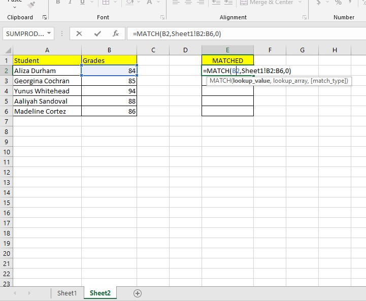
The MATCH function is a powerful tool for comparing data in two Excel sheets. It searches for a specified item in a range of cells and returns the relative position of that item in the range.

How it works: The MATCH function looks for a value in one sheet within a specified range in another sheet. If the value is found, MATCH returns its position; otherwise, it returns an error. This makes it easy to identify if a value exists in both sheets.

Example:

=MATCH(A2,Sheet2!A:A,0)

This formula searches for the value in cell A2 of the current sheet within column A of Sheet2. If a match is found, it returns the row number where the match occurs. If no match is found, it returns #N/A.

Benefits:

• Precise Matching: It finds exact matches, ensuring accuracy.
• Returns Position: Knowing the position of the match can be useful for further analysis.

Limitations:

• Exact Matches Only: It only works for exact matches and is case-sensitive.
• Single Column Search: It searches only in a single column or row.

1.2 Leveraging VLOOKUP For Value Retrieval And Comparison

VLOOKUP (Vertical Lookup) is another useful function for comparing data in two sheets. It searches for a value in the first column of a range and returns a value from a column to the right in the same row.

How it works: VLOOKUP looks for a value in one sheet and retrieves corresponding data from another sheet. If the value is found, VLOOKUP returns a related value from the specified column. If not found, it returns an error.

Example:

=VLOOKUP(A2,Sheet2!A:B,2,FALSE)

This formula searches for the value in cell A2 of the current sheet within column A of Sheet2, and if found, returns the value from the second column (B) in Sheet2. The FALSE argument ensures an exact match.

Benefits:

• Value Retrieval: It can retrieve associated data, allowing you to compare additional information.
• Flexible Search: It can search for values based on partial matches.

Limitations:

• Lookup Column Restriction: It only searches in the first column of the specified range.
• Error Handling: Requires error handling (e.g., using IFERROR) to manage cases where no match is found.

1.3 Utilizing COUNTIF To Identify Duplicates And Matches

The COUNTIF function counts the number of cells within a range that meet a given criterion. It’s useful for identifying duplicates and matches between two sheets.

How it works: COUNTIF counts how many times a value from one sheet appears in another sheet. This helps identify whether a value is unique to one sheet or present in both.

Example:

=COUNTIF(Sheet2!A:A,A2)

This formula counts how many times the value in cell A2 of the current sheet appears in column A of Sheet2. If the result is greater than 0, the value exists in both sheets.

Benefits:

• Simple Implementation: It’s easy to use and understand.
• Duplicate Detection: It can quickly identify duplicates within and between sheets.

Limitations:

• Basic Matching: It only counts occurrences and doesn’t provide additional information about the matches.
• No Differentiation: It doesn’t differentiate between exact and partial matches without additional criteria.

1.4 Conditional Formatting For Visual Matching

Conditional formatting allows you to highlight cells based on specific criteria. It’s a great way to visually identify matches and differences between two sheets.

How it works: By setting up rules in conditional formatting, you can highlight cells that meet certain conditions, such as matching values in another sheet.

Example:

1. Select the range of cells you want to compare in Sheet1.
2. Go to Conditional Formatting > New Rule.
3. Choose “Use a formula to determine which cells to format.”
4. Enter the formula: =COUNTIF(Sheet2!A:A,A1)>0.
5. Set the desired formatting (e.g., fill color) and click OK.

Benefits:

• Visual Identification: Easily spot matches and differences with color-coded highlights.
• Customizable: Flexible rules to highlight specific criteria.

Limitations:

• Manual Setup: Requires manual setup of rules and formatting.
• Performance: Can slow down Excel with large datasets.

1.5 Combining INDEX and MATCH for Advanced Comparisons

Combining the INDEX and MATCH functions offers a more flexible alternative to VLOOKUP. This combination allows you to look up values in any column and return corresponding values from any other column.

How it works: The MATCH function finds the row number of a value in a range, and the INDEX function returns the value in a specified row and column.

Example:

=INDEX(Sheet2!B:B,MATCH(A2,Sheet2!A:A,0))

This formula searches for the value in cell A2 of the current sheet within column A of Sheet2 and returns the corresponding value from column B in Sheet2.

Benefits:

• Flexible Lookup: Can look up values in any column and return corresponding values from any other column.
• Dynamic: Less prone to errors when columns are inserted or deleted.

Limitations:

• Complex Syntax: More complex syntax than VLOOKUP.
• Error Handling: Requires error handling to manage cases where no match is found.

2. How Do I Highlight The Matching Data From A Separate Worksheet Within The Same Workbook?

To highlight matching data from a separate worksheet within the same workbook, use conditional formatting with a formula that references the other sheet. Select the data range, create a new conditional formatting rule using a formula like =COUNTIF(Sheet2!A:A,A1)>0, and set the desired highlighting format. This will automatically highlight matching values.

Conditional formatting in Excel is a powerful feature that allows you to automatically apply formatting to cells based on specified criteria. When working with multiple worksheets in the same workbook, highlighting matching data can significantly improve data analysis and presentation. This section provides a step-by-step guide on how to achieve this.

2.1 Step-By-Step Guide To Highlighting Matches

Follow these steps to highlight matching data from a separate worksheet within the same workbook using conditional formatting:

Step 1: Select The Data Range

First, select the range of cells in the worksheet where you want to highlight the matching data. This is the range that will be formatted based on whether the values match those in another sheet.

Step 2: Open Conditional Formatting

Go to the Home tab on the Excel ribbon, then click on Conditional Formatting in the Styles group.

Step 3: Create A New Rule

From the dropdown menu, select New Rule. This will open the “New Formatting Rule” dialog box.

Step 4: Use A Formula To Determine Which Cells To Format

In the “New Formatting Rule” dialog box, choose the rule type “Use a formula to determine which cells to format”. This option allows you to use a formula to define the conditions for formatting.

Step 5: Enter The Formula

In the formula box, enter a formula that checks for matches in the other worksheet. A common formula for this purpose is:

=COUNTIF(Sheet2!A:A,A1)>0

This formula checks if the value in cell A1 of the current sheet exists in column A of Sheet2. If the COUNTIF function returns a value greater than 0, it means the value exists in Sheet2, and the conditional formatting will be applied.

Note: Adjust the formula based on the actual sheet name and data range you are comparing.

Step 6: Set The Formatting

Click the Format button to set the formatting you want to apply to the matching cells. You can change the font, border, fill color, and other formatting options.

Step 7: Apply The Rule

Click OK in both the “Format Cells” and “New Formatting Rule” dialog boxes to apply the rule.

Now, all cells in the selected range that have matching values in the specified range of the other worksheet will be highlighted with the formatting you selected.

2.2 Examples Of Different Formulas

Here are a few examples of different formulas you can use in conditional formatting to highlight matching data, depending on your specific needs:

2.2.1 Exact Match In A Single Column

=COUNTIF(Sheet2!A:A,A1)>0

This formula highlights cells in the current sheet if their values exist in column A of Sheet2.

2.2.2 Match In Multiple Columns

=OR(COUNTIF(Sheet2!A:A,A1)>0, COUNTIF(Sheet2!B:B,A1)>0)

This formula highlights cells if their values exist in either column A or column B of Sheet2.

2.2.3 Match Based On Multiple Criteria

=AND(COUNTIF(Sheet2!A:A,A1)>0, B1=Sheet2!B1)

This formula highlights cells if their values exist in column A of Sheet2 and if the value in column B of the current sheet matches the value in column B of Sheet2 for the same row.

2.3 Tips For Effective Conditional Formatting

• Use Absolute References: When defining the range in the formula, use absolute references (e.g., $A$1:$A$10) to prevent the range from changing when the conditional formatting is applied to other cells.
• Test The Formula: Before applying the conditional formatting, test the formula in a cell to ensure it returns the correct result.
• Manage Rules: Use the Conditional Formatting Rules Manager to edit, delete, or reorder rules.
• Consider Performance: Applying conditional formatting to large datasets can slow down Excel. Use it judiciously and optimize your formulas.

By following these steps and tips, you can effectively highlight matching data from a separate worksheet within the same Excel workbook. This can significantly improve your ability to analyze and present data accurately.

3. What Are Some Common Mistakes When Comparing Excel Sheets?

Common mistakes when comparing Excel sheets include incorrect formula syntax, inconsistent data formatting, overlooking case sensitivity, not using absolute references, and failing to handle errors. These errors can lead to inaccurate results and missed matches.

Comparing Excel sheets for matching data can be a complex process, and it’s easy to make mistakes that can lead to inaccurate results. Avoiding these common pitfalls can save time and ensure data integrity. This section highlights some of the most frequent errors and provides tips on how to prevent them.

3.1 Incorrect Formula Syntax

One of the most common mistakes is using incorrect syntax in Excel formulas. This can lead to errors or incorrect results when comparing data.

How it happens:

• Misspelled Function Names: For example, writing VLOKUP instead of VLOOKUP.
• Incorrect Arguments: Providing the wrong number or type of arguments to a function.
• Missing Parentheses or Commas: Forgetting to close parentheses or using incorrect separators.

How to avoid it:

• Double-Check Syntax: Always double-check the syntax of your formulas using Excel’s built-in help.
• Use Formula Auto-Complete: Excel’s auto-complete feature can help you enter function names and arguments correctly.
• Test Formulas: Test your formulas on a small sample of data to ensure they return the expected results.

3.2 Inconsistent Data Formatting

Inconsistent data formatting can cause Excel to misidentify matches, leading to inaccurate comparisons.

How it happens:

• Different Date Formats: Dates formatted as MM/DD/YYYY in one sheet and DD/MM/YYYY in another.
• Number Formatting: Numbers stored as text or with different decimal places.
• Leading or Trailing Spaces: Extra spaces before or after text values.

How to avoid it:

• Standardize Data Formats: Ensure all data in both sheets is formatted consistently. Use Excel’s formatting tools to standardize date, number, and text formats.
• Trim Spaces: Use the TRIM function to remove leading and trailing spaces from text values.
• Check Data Types: Verify that numbers are stored as numbers and not as text. You can use the ISTEXT or ISNUMBER functions to check data types.

3.3 Overlooking Case Sensitivity

Excel functions like VLOOKUP and MATCH are case-insensitive by default. This means that “Apple” and “apple” are treated as the same value, which can lead to incorrect matches in certain cases.

How it happens:

• Mismatched Case: Data in one sheet has different capitalization than in another.

How to avoid it:

• Use Case-Sensitive Formulas: Use functions like EXACT to perform case-sensitive comparisons. For example:

  =IF(EXACT(A1,Sheet2!A1), "Match", "No Match")

• Standardize Case: Use the UPPER, LOWER, or PROPER functions to standardize the case of text values before comparing.

3.4 Not Using Absolute References

When using formulas that refer to specific ranges in other sheets, it’s important to use absolute references ($) to prevent the references from changing when the formula is copied to other cells.

How it happens:

• Relative References: Using relative references (e.g., A1) instead of absolute references (e.g., $A$1) can cause the formula to refer to the wrong cells when copied.

How to avoid it:

• Use Absolute References: Always use absolute references when referring to fixed ranges in your formulas. For example:

  =VLOOKUP(A1,Sheet2!$A$1:$B$100,2,FALSE)

3.5 Failing To Handle Errors

When comparing data, it’s common to encounter errors, such as #N/A when a value is not found. Failing to handle these errors can lead to misleading results.

How it happens:

• Unaccounted Errors: Errors in formulas are not handled, causing the entire comparison to fail.

How to avoid it:

• Use Error Handling Functions: Use functions like IFERROR or ISERROR to handle errors gracefully. For example:

  =IFERROR(VLOOKUP(A1,Sheet2!A:B,2,FALSE), "Not Found")

  This formula returns “Not Found” if the VLOOKUP function returns an error.

3.6 Ignoring Hidden Rows Or Columns

Hidden rows or columns can contain data that affects the comparison results. Ignoring them can lead to inaccurate conclusions.

How it happens:

• Omitted Data: Hidden rows or columns contain data that is not included in the comparison.

How to avoid it:

• Unhide Rows and Columns: Before comparing data, unhide all rows and columns in both sheets to ensure all data is included.

3.7 Using Incompatible Data Types

Comparing data with incompatible data types (e.g., text vs. number) can lead to incorrect matches.

How it happens:

• Mixed Data Types: Comparing a text value with a number value, or a date value with a text value.

How to avoid it:

• Convert Data Types: Use functions like VALUE, TEXT, or DATEVALUE to convert data to compatible data types before comparing. For example:

  =IF(VALUE(A1)=B1, "Match", "No Match")

By avoiding these common mistakes, you can ensure more accurate and reliable results when comparing Excel sheets for matching data.

4. What Formulas Can I Use For Matching Values In Microsoft Excel?

Several formulas can be used for matching values in Microsoft Excel, including MATCH, VLOOKUP, COUNTIF, INDEX/MATCH, and SUMIF. The MATCH function finds the position of a value, VLOOKUP retrieves corresponding data, COUNTIF counts occurrences, INDEX/MATCH offers flexible lookup, and SUMIF sums values based on matching criteria.

Microsoft Excel offers a variety of formulas that can be used for matching values across different sheets or within the same sheet. Each formula has its own strengths and is suitable for different scenarios. This section will explore several key formulas, providing examples and use cases to help you choose the best one for your needs.

4.1 The MATCH Function

The MATCH function is used to find the position of a specific value within a range of cells. It returns the relative position of the matched item in the range.

Syntax:

=MATCH(lookup_value, lookup_array, [match_type])

• lookup_value: The value you want to find.
• lookup_array: The range of cells to search in.
• match_type: Optional. Specifies the type of match:
  • 0: Exact match (the most common).
  • 1: Finds the largest value that is less than or equal to lookup_value (requires the lookup_array to be sorted in ascending order).
  • -1: Finds the smallest value that is greater than or equal to lookup_value (requires the lookup_array to be sorted in descending order).

Example:

=MATCH("Apple", A1:A10, 0)

This formula searches for the value “Apple” in the range A1:A10 and returns its position. If “Apple” is found in cell A3, the formula will return 3.

Use Case:

• Finding the row number of a specific item in a list.
• Combining with other functions like INDEX for more complex lookups.

4.2 The VLOOKUP Function

The VLOOKUP (Vertical Lookup) function searches for a value in the first column of a range and returns a value from a column to the right in the same row.

Syntax:

=VLOOKUP(lookup_value, table_array, col_index_num, [range_lookup])

• lookup_value: The value you want to find.
• table_array: The range of cells to search in (the first column is where the lookup_value is searched).
• col_index_num: The column number in the table_array from which to return a value.
• range_lookup: Optional. Specifies whether to find an exact match or an approximate match:
  • TRUE or omitted: Approximate match (requires the first column of table_array to be sorted in ascending order).
  • FALSE: Exact match (recommended for most cases).

Example:

=VLOOKUP("Apple", A1:B10, 2, FALSE)

This formula searches for “Apple” in the first column of the range A1:B10 and returns the value from the second column in the same row where “Apple” is found.

Use Case:

• Retrieving associated data based on a lookup value.
• Combining data from multiple tables.

4.3 The COUNTIF Function

The COUNTIF function counts the number of cells within a range that meet a given criterion. It’s useful for checking if a value exists in a range.

Syntax:

=COUNTIF(range, criteria)

• range: The range of cells to count.
• criteria: The condition that determines which cells will be counted.

Example:

=COUNTIF(A1:A10, "Apple")

This formula counts the number of cells in the range A1:A10 that contain the value “Apple”.

Use Case:

• Checking if a value exists in a list.
• Counting the number of occurrences of a specific value.

4.4 Combining INDEX and MATCH

Combining the INDEX and MATCH functions provides a more flexible alternative to VLOOKUP. This combination allows you to look up values in any column and return corresponding values from any other column.

Syntax:

=INDEX(array, MATCH(lookup_value, lookup_array, [match_type]))

• array: The range of cells from which to return a value.
• MATCH(lookup_value, lookup_array, [match_type]): Returns the row number of the lookup_value in the lookup_array.

Example:

=INDEX(B1:B10, MATCH("Apple", A1:A10, 0))

This formula searches for “Apple” in the range A1:A10 and returns the corresponding value from the range B1:B10.

Use Case:

• Performing lookups in any direction (left, right, above, below).
• Creating dynamic lookup formulas that are less prone to errors when columns are inserted or deleted.

4.5 The SUMIF Function

The SUMIF function sums the values in a range that meet a given criterion. It can be used to sum values based on matching criteria in another range.

Syntax:

=SUMIF(range, criteria, [sum_range])

• range: The range of cells to evaluate.
• criteria: The condition that determines which cells will be summed.
• sum_range: Optional. The range of cells to sum. If omitted, the range is summed.

Example:

=SUMIF(A1:A10, "Apple", B1:B10)

This formula sums the values in the range B1:B10 where the corresponding cell in the range A1:A10 contains the value “Apple”.

Use Case:

• Summing values based on specific criteria.
• Calculating totals for specific categories.

4.6 Examples and Use Cases

Here are some additional examples and use cases for these formulas:

• Example 1: Finding a Customer ID in a List

  =MATCH(C2, CustomerIDs, 0)

  Where C2 contains the customer ID to search for and CustomerIDs is a named range containing a list of customer IDs.

• Example 2: Retrieving a Product Price

  =VLOOKUP(D2, ProductsTable, 3, FALSE)

  Where D2 contains the product name, ProductsTable is a range containing product data, and 3 is the column number containing the price.

• Example 3: Counting Orders for a Specific Product

  =COUNTIF(OrdersTable[Product], "Laptop")

  Where OrdersTable[Product] is a structured reference to the “Product” column in a table named “OrdersTable”.

By understanding and using these formulas, you can effectively match values in Microsoft Excel and perform a wide range of data analysis tasks.

5. How Can I Compare Two Excel Sheets For Differences?

To compare two Excel sheets for differences, use conditional formatting to highlight discrepancies, or use formulas like IF and NOT(EXACT()) to identify non-matching cells. Excel also offers built-in tools like “Compare Side by Side” and third-party add-ins for more comprehensive comparisons.

Comparing two Excel sheets to identify differences is a crucial task in data management and analysis. Several methods can be employed to effectively highlight discrepancies. This section explores the most useful techniques for comparing two Excel sheets and pinpointing differences.

5.1 Using Conditional Formatting To Highlight Differences

Conditional formatting can be used to highlight cells that have different values in two Excel sheets. This method provides a visual way to quickly identify discrepancies.

How it works:

1. Select the Range: Select the range of cells you want to compare in one sheet.
2. Create a New Rule: Go to Conditional Formatting > New Rule.
3. Use a Formula: Choose “Use a formula to determine which cells to format.”
4. Enter the Formula: Enter a formula that compares the selected cell with the corresponding cell in the other sheet. For example:

=A1<>Sheet2!A1

5. Set the Formatting: Click the Format button to set the formatting (e.g., fill color) for the cells that meet the criteria.
6. Apply the Rule: Click OK in both dialog boxes to apply the rule.

Benefits:

• Visual Identification: Easily spot differences with color-coded highlights.
• Customizable: Flexible rules to highlight specific criteria.

Limitations:

• Manual Setup: Requires manual setup of rules and formatting.
• Performance: Can slow down Excel with large datasets.

5.2 Using Formulas To Identify Non-Matching Cells

Excel formulas can be used to identify non-matching cells by comparing values directly and returning a result based on whether they match or not.

How it works:

1. Use the IF Function: Use the IF function to compare values in two cells.
2. Compare Values: Compare the selected cell with the corresponding cell in the other sheet. For example:

=IF(A1=Sheet2!A1, "Match", "Difference")

3. Display Results: The formula will display “Match” if the values are the same and “Difference” if they are different.

Benefits:

• Clear Results: Provides clear text-based results.
• Easy to Understand: Simple and easy to understand formulas.

Limitations:

• Requires Extra Columns: Requires additional columns to display the results.
• Manual Setup: Requires manual setup for each comparison.

5.3 Using the NOT(EXACT()) Function For Case-Sensitive Comparisons

For case-sensitive comparisons, the NOT(EXACT()) function can be used to identify differences in text values.

How it works:

1. Use the EXACT Function: The EXACT function compares two text strings and returns TRUE if they are exactly the same (including case) and FALSE otherwise.
2. Use the NOT Function: The NOT function reverses the result of the EXACT function.
3. Combine the Functions: Combine the NOT and EXACT functions to identify differences:

=IF(NOT(EXACT(A1,Sheet2!A1)), "Case Difference", "Match")

Benefits:

• Case-Sensitive: Identifies differences in text case.
• Precise Matching: Ensures exact matching.

Limitations:

• Text Values Only: Works only for text values.
• Requires Extra Columns: Requires additional columns to display the results.

5.4 Using Excel’s “Compare Side by Side” Feature

Excel’s “Compare Side by Side” feature allows you to view two sheets simultaneously and scroll them in sync to easily compare their contents.

How it works:

1. Open Both Sheets: Open both Excel sheets you want to compare.

2. Go to View Tab: Click on the View tab in the Excel ribbon.

3. Click Compare Side by Side: In the Window group, click Compare Side by Side.

4. Synchronous Scrolling: Excel will display both sheets side by side and enable synchronous scrolling, allowing you to scroll through both sheets at the same time.

Benefits:

• Simultaneous Viewing: Allows you to view both sheets at the same time.
• Synchronous Scrolling: Enables synchronous scrolling for easy comparison.

Limitations:

• Manual Comparison: Requires manual visual comparison.
• Limited Automation: Does not automatically highlight differences.

5.5 Using Third-Party Add-Ins

Several third-party add-ins are available for Excel that provide more advanced comparison features, such as detailed reports and automatic highlighting of differences.

How it works:

1. Install the Add-In: Install a third-party add-in for Excel.
2. Use the Add-In: Use the add-in to compare the two sheets and generate a report of the differences.

Benefits:

• Advanced Features: Provides advanced comparison features, such as detailed reports and automatic highlighting of differences.
• Automation: Automates the comparison process.

Limitations:

• Cost: May require purchasing a license.
• Compatibility: May not be compatible with all versions of Excel.

6. How Do I Ensure Data Consistency When Comparing Excel Sheets?

To ensure data consistency when comparing Excel sheets, standardize data formatting, remove duplicates, validate data entries, use absolute references in formulas, handle errors, and regularly audit your data. These practices help maintain accuracy and reliability in your comparisons.

Ensuring data consistency is crucial when comparing Excel sheets to make accurate assessments. Inconsistencies can lead to incorrect results and flawed decision-making. This section outlines the key steps to ensure data consistency when comparing Excel sheets.

6.1 Standardize Data Formatting

Inconsistent data formatting is a common issue that can lead to inaccurate comparisons. Standardizing data formatting ensures that values are recognized correctly.

How to do it:

1. Select the Range: Select the range of cells you want to format.
2. Use the Format Cells Dialog: Right-click and choose Format Cells.
3. Choose the Appropriate Format: Select the appropriate format (e.g., Date, Number, Text) and set the desired options.

Best Practices:

• Dates: Use a consistent date format (e.g., MM/DD/YYYY or DD/MM/YYYY).
• Numbers: Specify the number of decimal places and use consistent separators.
• Text: Remove leading and trailing spaces using the TRIM function.

6.2 Remove Duplicates

Duplicates can skew comparison results, especially when counting or summing values. Removing duplicates ensures that each unique value is considered only once.

How to do it:

1. Select the Range: Select the range of cells you want to check for duplicates.
2. Go to Data Tab: Click on the Data tab in the Excel ribbon.
3. Click Remove Duplicates: In the Data Tools group, click Remove Duplicates.
4. Select Columns: Select the columns you want to check for duplicates and click OK.

Best Practices:

• Review Duplicates: Review the duplicates before removing them to ensure you are not deleting important data.
• Backup Data: Create a backup of your data before removing duplicates.

6.3 Validate Data Entries

Data validation helps prevent inconsistent entries by restricting the type of data that can be entered into a cell.

How to do it:

1. Select the Range: Select the range of cells you want to validate.
2. Go to Data Tab: Click on the Data tab in the Excel ribbon.
3. Click Data Validation: In the Data Tools group, click Data Validation.
4. Set Validation Criteria: Set the validation criteria (e.g., Whole number, Decimal, List, Date, Time, Text length) and specify the desired options.

Best Practices:

• Use Dropdown Lists: Use dropdown lists for predefined values to ensure consistency.
• Set Input Messages: Set input messages to provide guidance to users.
• Set Error Alerts: Set error alerts to notify users when they enter invalid data.

6.4 Use Absolute References In Formulas

When using formulas that refer to specific ranges in other sheets, it’s important to use absolute references ($) to prevent the references from changing when the formula is copied to other cells.

How to do it:

• Use Absolute References: Always use absolute references when referring to fixed ranges in your formulas. For example:

  =VLOOKUP(A1,Sheet2!$A$1:$B$100,2,FALSE)

6.5 Handle Errors Gracefully

When comparing data, it’s common to encounter errors, such as #N/A when a value is not found. Handling these errors gracefully prevents them from disrupting the comparison process.

How to do it:

• Use Error Handling Functions: Use functions like IFERROR or ISERROR to handle errors gracefully. For example:

  =IFERROR(VLOOKUP(A1,Sheet2!A:B,2,FALSE), "Not Found")