How to Compare Two Excel Sheets Data Using VLOOKUP

Comparing two sets of data in Excel can be a daunting task, especially when dealing with large spreadsheets. At COMPARE.EDU.VN, we understand the need for efficient data comparison methods. This article will guide you through How To Compare Two Excel Sheets Data Using Vlookup, a powerful function that simplifies the reconciliation process. This method ensures accuracy and saves valuable time, making data comparison and Excel data analysis more manageable.

Table of Contents

1. Introduction to Data Comparison in Excel
2. Understanding VLOOKUP Function
3. Step-by-Step Guide: How to Compare Two Excel Sheets Data Using VLOOKUP
   • 3.1. Setting Up Your Data
   • 3.2. Applying the VLOOKUP Formula
   • 3.3. Interpreting VLOOKUP Results
4. Advanced Techniques for Data Reconciliation
   • 4.1. Using IF and ISERROR Functions
   • 4.2. Conditional Formatting for Highlighting Differences
5. Alternative Methods for Comparing Excel Sheets
   • 5.1. Using XLOOKUP Function
   • 5.2. Utilizing Excel’s Built-in Comparison Tools
6. Best Practices for Accurate Data Comparison
7. Troubleshooting Common Issues with VLOOKUP
8. Real-World Applications of Excel Data Comparison
9. COMPARE.EDU.VN: Your Partner in Data Analysis
10. Frequently Asked Questions (FAQs)
11. Conclusion

1. Introduction to Data Comparison in Excel

Data comparison is a crucial task in various fields, from finance and accounting to marketing and sales. Whether you’re reconciling financial statements, comparing sales data from different periods, or identifying discrepancies in customer databases, the ability to accurately compare data is essential. Excel, with its versatile functions and tools, offers several methods for comparing data, but VLOOKUP stands out as a particularly efficient and effective solution. This article will explore how to leverage the VLOOKUP function to streamline your data comparison tasks, enhancing your proficiency in data reconciliation and validation. Comparing datasets can be a complex process, but with the right techniques, it becomes manageable and insightful.

2. Understanding VLOOKUP Function

The VLOOKUP function is a fundamental tool in Excel for searching for a specific value in a table and returning a corresponding value from another column in the same row. It’s particularly useful when you need to compare data across two different Excel sheets based on a common identifier, such as a customer ID, product code, or invoice number. The VLOOKUP function operates by searching for the lookup value in the first column of a specified table range and then retrieving a value from a column you designate. This function is invaluable for tasks like matching data, identifying missing entries, and comparing values across different datasets. Understanding the syntax and parameters of VLOOKUP is essential for effective data comparison.

The syntax for the VLOOKUP function is as follows:

=VLOOKUP(lookup_value, table_array, col_index_num, [range_lookup])

• lookup_value: The value you want to search for in the first column of the table array.
• table_array: The range of cells that contains the data you want to search.
• col_index_num: The column number in the table array from which you want to retrieve a value.
• range_lookup: An optional argument that specifies whether you want to find an exact match (FALSE) or an approximate match (TRUE). For most data comparison tasks, you’ll want to use FALSE to ensure accuracy.

3. Step-by-Step Guide: How to Compare Two Excel Sheets Data Using VLOOKUP

Here’s a detailed guide on how to compare two Excel sheets using VLOOKUP:

3.1. Setting Up Your Data

Before you can use VLOOKUP, you need to ensure that your data is properly organized in the two Excel sheets you want to compare.

1. Open Your Excel File: Open the Excel file containing the two sheets you want to compare. For example, you might have two sheets named “Sheet1” and “Sheet2”.
2. Identify a Common Identifier: Identify a column that contains a unique identifier common to both sheets. This could be a customer ID, product code, invoice number, or any other unique value that appears in both datasets.
3. Arrange Your Data: Ensure that the common identifier is in the first column of the table array in both sheets. If it’s not, you may need to rearrange your columns.
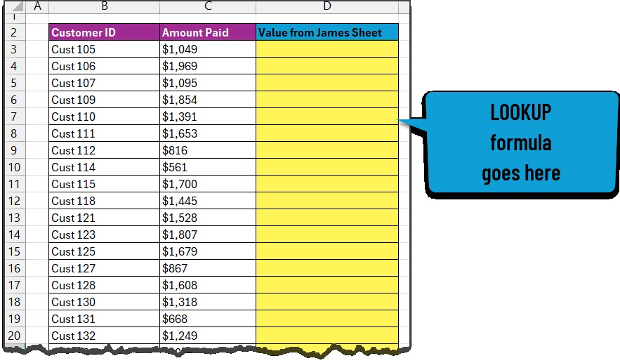
4. Create New Columns: In the first sheet, insert a new column next to the column containing the common identifier. This column will be used to display the corresponding values from the second sheet.

For instance, suppose you have two sheets, “SalesData1” and “SalesData2,” both containing sales records. Each record includes a “ProductID,” “ProductName,” and “SalesAmount.” You want to compare the “SalesAmount” in both sheets for each product.

3.2. Applying the VLOOKUP Formula

Now that your data is set up, you can apply the VLOOKUP formula to compare the data in the two sheets.

1. Select the First Cell: In the first sheet (“SalesData1”), select the first cell in the new column you created (e.g., D2).
2. Enter the VLOOKUP Formula: Enter the VLOOKUP formula in the selected cell. The formula will look something like this:

=VLOOKUP(A2,SalesData2!A:C,3,FALSE)

In this formula:

• A2: Is the lookup value, which is the “ProductID” in the first row of “SalesData1.”
• SalesData2!A:C: Is the table array, which is the range of cells in “SalesData2” that contains the “ProductID,” “ProductName,” and “SalesAmount.”
• 3: Is the column index number, which specifies that you want to retrieve the value from the third column (“SalesAmount”) in the table array.
• FALSE: Specifies that you want to find an exact match for the lookup value.

3. Copy the Formula: Drag the fill handle (the small square at the bottom-right corner of the cell) down to apply the formula to all the rows in the first sheet.

3.3. Interpreting VLOOKUP Results

After applying the VLOOKUP formula, you’ll see the corresponding “SalesAmount” from “SalesData2” in the new column in “SalesData1.” If a “ProductID” exists in “SalesData1” but not in “SalesData2,” the VLOOKUP function will return an #N/A error.

1. Identify Matches and Discrepancies: Compare the “SalesAmount” values in “SalesData1” with the corresponding values retrieved from “SalesData2.” If the values are the same, it means the sales amounts match for that product. If the values are different, it indicates a discrepancy that needs further investigation.
2. Handle #N/A Errors: The #N/A errors indicate that the “ProductID” is missing in “SalesData2.” This could be due to various reasons, such as data entry errors or products being discontinued.

4. Advanced Techniques for Data Reconciliation

To enhance the data comparison process, you can use additional Excel functions and features:

4.1. Using IF and ISERROR Functions

To handle #N/A errors and provide more informative results, you can combine the VLOOKUP function with the IF and ISERROR functions.

1. Modify the Formula: Modify the VLOOKUP formula to include the IF and ISERROR functions:

=IF(ISERROR(VLOOKUP(A2,SalesData2!A:C,3,FALSE)),"Missing",VLOOKUP(A2,SalesData2!A:C,3,FALSE))

In this modified formula:

• ISERROR(VLOOKUP(A2,SalesData2!A:C,3,FALSE)): Checks if the VLOOKUP function returns an error (#N/A).
• “Missing”: If the VLOOKUP function returns an error, the formula will display “Missing.”
• VLOOKUP(A2,SalesData2!A:C,3,FALSE): If the VLOOKUP function does not return an error, the formula will display the corresponding “SalesAmount” from “SalesData2.”

2. Compare Values: To compare the “SalesAmount” values and identify discrepancies, use the IF function:

=IF(ISERROR(VLOOKUP(A2,SalesData2!A:C,3,FALSE)),"Missing",IF(C2=VLOOKUP(A2,SalesData2!A:C,3,FALSE),"Match","Mismatch"))

In this formula:

• C2: Is the “SalesAmount” in “SalesData1.”
• VLOOKUP(A2,SalesData2!A:C,3,FALSE): Is the corresponding “SalesAmount” from “SalesData2.”
• “Match”: If the “SalesAmount” values are the same, the formula will display “Match.”
• “Mismatch”: If the “SalesAmount” values are different, the formula will display “Mismatch.”

4.2. Conditional Formatting for Highlighting Differences

Conditional formatting can be used to visually highlight the differences between the two sheets.

1. Select the Range: Select the range of cells containing the comparison results (e.g., D2:D100).
2. Open Conditional Formatting: Go to the “Home” tab in the Excel ribbon and click on “Conditional Formatting” in the “Styles” group.
3. Create a New Rule: Select “New Rule” from the dropdown menu.
4. Choose a Rule Type: In the “New Formatting Rule” dialog box, select “Use a formula to determine which cells to format.”
5. Enter the Formula: Enter the following formula:

=$D2="Mismatch"

1. Set the Format: Click on the “Format” button and choose a formatting style (e.g., fill color, font color) to highlight the mismatched values.
2. Add Another Rule: Repeat the steps to add another rule to highlight the “Missing” values. Use the following formula:

=$D2="Missing"

5. Alternative Methods for Comparing Excel Sheets

While VLOOKUP is a powerful tool, there are alternative methods for comparing data in Excel.

5.1. Using XLOOKUP Function

XLOOKUP is a modern alternative to VLOOKUP that offers several advantages, including improved flexibility and ease of use.

1. Syntax: The syntax for the XLOOKUP function is as follows:

=XLOOKUP(lookup_value, lookup_array, return_array, [if_not_found], [match_mode], [search_mode])

• lookup_value: The value you want to search for.
• lookup_array: The range of cells to search within.
• return_array: The range of cells from which to return a value.
• if_not_found: An optional argument that specifies the value to return if no match is found.
• match_mode: An optional argument that specifies the type of match to perform (e.g., exact match, wildcard match).
• search_mode: An optional argument that specifies the search direction (e.g., first to last, last to first).

2. Example: To compare the “SalesAmount” in “SalesData1” and “SalesData2” using XLOOKUP, you would use the following formula:

=XLOOKUP(A2,SalesData2!A:A,SalesData2!C:C,"Missing")

In this formula:

• A2: Is the lookup value, which is the “ProductID” in the first row of “SalesData1.”
• SalesData2!A:A: Is the lookup array, which is the range of cells in “SalesData2” that contains the “ProductID.”
• SalesData2!C:C: Is the return array, which is the range of cells in “SalesData2” that contains the “SalesAmount.”
• “Missing”: Is the value to return if no match is found.

5.2. Utilizing Excel’s Built-in Comparison Tools

Excel also offers built-in comparison tools that can be used to compare data in two sheets.

1. Inquire Tab: If you have Excel Professional Plus, you can use the Inquire tab to compare two workbooks. This tab provides tools for analyzing and comparing workbooks, identifying differences, and highlighting potential issues.
2. View Side by Side: You can use the “View Side by Side” feature to view two sheets or workbooks at the same time, making it easier to compare data manually.
3. Go to View Tab: Click “View Side by Side” in the Window group. Excel will arrange the two windows on the screen so you can compare them.

6. Best Practices for Accurate Data Comparison

To ensure accurate data comparison, follow these best practices:

• Verify Data Integrity: Before comparing data, verify that the data in both sheets is accurate and complete. Check for data entry errors, missing values, and inconsistencies.
• Standardize Data: Standardize the data in both sheets to ensure that it is consistent. This includes formatting dates, numbers, and text.
• Use Unique Identifiers: Use unique identifiers to match records in the two sheets. This will help ensure that you are comparing the correct data.
• Test Your Formulas: Before applying your formulas to the entire dataset, test them on a small sample to ensure that they are working correctly.
• Document Your Process: Document your data comparison process so that you can easily repeat it in the future.

7. Troubleshooting Common Issues with VLOOKUP

When using VLOOKUP, you may encounter some common issues:

• #N/A Errors: The #N/A error indicates that the lookup value was not found in the table array. This could be due to various reasons, such as data entry errors, missing values, or incorrect lookup values.
• Incorrect Results: If you are getting incorrect results, double-check your formulas to ensure that you are using the correct lookup value, table array, and column index number.
• Performance Issues: If you are working with large datasets, VLOOKUP can be slow. To improve performance, try sorting your data and using the INDEX and MATCH functions instead of VLOOKUP.
• Inconsistent Data Types: Ensure that the data types of the lookup value and the values in the first column of the table array are consistent. For example, if the lookup value is a number, the values in the first column of the table array should also be numbers.

8. Real-World Applications of Excel Data Comparison

Excel data comparison has numerous real-world applications across various industries:

• Finance: Reconciling financial statements, comparing budget vs. actual expenses, and identifying fraudulent transactions.
• Accounting: Auditing financial records, comparing invoices with purchase orders, and verifying vendor payments.
• Marketing: Comparing sales data from different periods, analyzing customer demographics, and measuring the effectiveness of marketing campaigns.
• Sales: Tracking sales performance, comparing sales forecasts with actual sales, and identifying sales trends.
• Human Resources: Comparing employee data, tracking employee performance, and managing payroll.
• Healthcare: Analyzing patient data, tracking medical outcomes, and managing healthcare costs.
• Education: Comparing student performance, tracking student attendance, and managing academic records.

By mastering Excel data comparison techniques, you can improve your efficiency, accuracy, and decision-making in these and other fields.

9. COMPARE.EDU.VN: Your Partner in Data Analysis

At COMPARE.EDU.VN, we are dedicated to providing you with the tools and knowledge you need to excel in data analysis. Our website offers a wide range of resources, including tutorials, articles, and templates, to help you master Excel and other data analysis tools. Whether you are a beginner or an experienced professional, we have something to help you improve your skills and advance your career. We strive to offer unbiased and comprehensive comparisons to assist you in making informed decisions. Explore our resources today and discover how we can help you unlock the full potential of your data.

Need more comparisons? Visit COMPARE.EDU.VN today for comprehensive and objective analysis. Let us help you make the best choices. Our address is 333 Comparison Plaza, Choice City, CA 90210, United States. Contact us via Whatsapp at +1 (626) 555-9090.

10. Frequently Asked Questions (FAQs)

Q1: What is the VLOOKUP function in Excel?

A: VLOOKUP is an Excel function used to search for a value in the first column of a table and return a corresponding value from another column in the same row.

Q2: How do I use VLOOKUP to compare two Excel sheets?

A: You can use VLOOKUP to compare two Excel sheets by using a common identifier to match records in the two sheets and compare the corresponding values.

Q3: What does the #N/A error mean in VLOOKUP?

A: The #N/A error indicates that the lookup value was not found in the table array. This could be due to various reasons, such as data entry errors or missing values.

Q4: How can I handle #N/A errors in VLOOKUP?

A: You can handle #N/A errors by using the IF and ISERROR functions to display a more informative message, such as “Missing” or “Not Found.”

Q5: What is the difference between VLOOKUP and XLOOKUP?

A: XLOOKUP is a modern alternative to VLOOKUP that offers several advantages, including improved flexibility and ease of use.

Q6: Can I use VLOOKUP to compare data in two different workbooks?

A: Yes, you can use VLOOKUP to compare data in two different workbooks by specifying the full path to the table array in the VLOOKUP formula.

Q7: How can I improve the performance of VLOOKUP when working with large datasets?

A: To improve the performance of VLOOKUP, try sorting your data and using the INDEX and MATCH functions instead of VLOOKUP.

Q8: What are some best practices for accurate data comparison in Excel?

A: Some best practices include verifying data integrity, standardizing data, using unique identifiers, testing your formulas, and documenting your process.

Q9: What are some real-world applications of Excel data comparison?

A: Excel data comparison has numerous real-world applications across various industries, including finance, accounting, marketing, sales, human resources, healthcare, and education.

Q10: Where can I find more resources to help me master Excel data comparison?

A: You can find more resources on COMPARE.EDU.VN, which offers a wide range of tutorials, articles, and templates to help you master Excel and other data analysis tools.

11. Conclusion

In conclusion, comparing two Excel sheets data using VLOOKUP is an efficient and effective way to reconcile data, identify discrepancies, and ensure accuracy. By following the step-by-step guide and best practices outlined in this article, you can streamline your data comparison tasks and improve your decision-making. Remember to leverage the power of Excel’s functions and features, and don’t hesitate to explore alternative methods to find the best solution for your needs. With practice and dedication, you can master Excel data comparison and unlock the full potential of your data. Remember to visit compare.edu.vn for more resources and tools to help you excel in data analysis.