**How to Compare Two Excel Columns Using VLOOKUP: A Comprehensive Guide**

Comparing two Excel columns using VLOOKUP is a common task for data analysis and manipulation. COMPARE.EDU.VN provides a detailed guide on how to effectively use VLOOKUP to identify matches and differences between columns. Master VLOOKUP for efficient data comparison, data matching and error handling.

1. What is VLOOKUP and Why Use it to Compare Excel Columns?

VLOOKUP (Vertical Lookup) is a powerful function in Excel used to find a value in the first column of a range and return a value in the same row from another column.
VLOOKUP can be used to:

• Identify common values: Determine which values exist in both columns.
• Find missing values: Locate data points that are present in one column but not the other.
• Return related data: Retrieve corresponding information from another column based on a match.

2. Understanding the VLOOKUP Syntax

The syntax of the VLOOKUP function is as follows:

=VLOOKUP(lookup_value, table_array, col_index_num, [range_lookup])

Let’s break down each argument:

• lookup_value: The value you want to search for in the first column of the table array.
• table_array: The range of cells that contains the data you want to search through. The first column of this range is where the lookup value will be searched.
• col_index_num: The column number within the table array that contains the value you want to return.
• range_lookup: An optional argument that specifies whether you want an exact or approximate match.
  • TRUE (or omitted): Approximate match. VLOOKUP will return the closest match less than or equal to the lookup value. The first column of the table array must be sorted in ascending order.
  • FALSE: Exact match. VLOOKUP will only return a value if it finds an exact match for the lookup value.

Important Notes:

• VLOOKUP only searches in the first column of the table_array.
• When using range_lookup = TRUE, ensure your data is sorted in ascending order to avoid incorrect results.
• If VLOOKUP doesn’t find an exact match with range_lookup = FALSE, it returns a #N/A error.

3. Basic VLOOKUP Formula to Compare Two Columns

This section will guide you through constructing a basic VLOOKUP formula to compare two columns in Excel.

3.1. Scenario:

Imagine you have two lists:

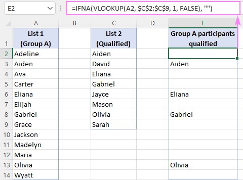
• List 1 (Column A): Names of participants in a competition.
• List 2 (Column C): Names of participants who qualified for the final round.

Your goal is to determine which participants from List 1 made it to the final round (i.e., their names are also present in List 2).

3.2. The Formula:

=VLOOKUP(A2, $C$2:$C$9, 1, FALSE)

3.3. Explanation:

• A2: This is the lookup_value. It refers to the first cell in List 1 (the name of the first participant).
• $C$2:$C$9: This is the table_array. It represents the entire List 2, where we’ll search for the participant’s name. The dollar signs ($) create absolute references, ensuring that the range remains fixed when you copy the formula down.
• 1: This is the col_index_num. Since List 2 only has one column, we use 1 to indicate that we want to return the value from that column.
• FALSE: This is the range_lookup. We use FALSE to specify that we want an exact match.

3.4. How to Use the Formula:

1. Enter the formula in cell E2 (or any empty column next to List 1).
2. Press Enter. The formula will search for the name in A2 within List 2 (C2:C9).
   • If the name is found in List 2, the formula will return the name itself.
   • If the name is not found, the formula will return a #N/A error.
3. Drag the fill handle (the small square at the bottom-right corner of the cell) down to apply the formula to all the names in List 1.

3.5. Interpreting the Results:

• Name displayed in Column E: The participant from List 1 is also present in List 2 (they qualified).
• #N/A error in Column E: The participant from List 1 is not present in List 2 (they did not qualify).

4. Handling #N/A Errors with IFNA and IFERROR

The #N/A errors returned by VLOOKUP can be unsightly and confusing. To improve the readability of your results, you can use the IFNA or IFERROR functions to replace these errors with more user-friendly values.

4.1. Using IFNA (Excel 2013 and later):

The IFNA function allows you to specify a value to return if a formula results in a #N/A error.

Syntax:

=IFNA(value, value_if_na)

• value: The formula you want to evaluate (in this case, your VLOOKUP formula).
• value_if_na: The value you want to return if the formula results in a #N/A error.

Example:

=IFNA(VLOOKUP(A2, $C$2:$C$9, 1, FALSE), "")

This formula will:

1. Perform the VLOOKUP as before.
2. If the VLOOKUP returns a #N/A error, IFNA will replace it with an empty string (“”), resulting in a blank cell.

You can replace the empty string with any other value you prefer, such as “Not Qualified” or “Not Found.”

=IFNA(VLOOKUP(A2, $C$2:$C$9, 1, FALSE), "Not in List 2")

4.2. Using IFERROR (Excel 2007 and later):

The IFERROR function is similar to IFNA but handles all types of errors, not just #N/A.

Syntax:

=IFERROR(value, value_if_error)

• value: The formula you want to evaluate (your VLOOKUP formula).
• value_if_error: The value you want to return if the formula results in any error.

Example:

=IFERROR(VLOOKUP(A2, $C$2:$C$9, 1, FALSE), "")

This formula will:

1. Perform the VLOOKUP.
2. If the VLOOKUP returns any error (including #N/A), IFERROR will replace it with an empty string.

Choosing Between IFNA and IFERROR:

• Use IFNA if you specifically want to handle #N/A errors and leave other errors untouched.
• Use IFERROR if you want to handle all errors in the same way. Be cautious when using IFERROR, as it can mask other potential errors in your formula that you might want to be aware of.

5. Comparing Columns in Different Excel Sheets

Often, the columns you need to compare reside in different worksheets within the same Excel file. VLOOKUP can easily handle this scenario using external references.

5.1. Scenario:

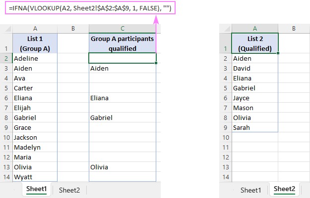
• Sheet1 (Column A): Contains List 1 (e.g., customer names).
• Sheet2 (Column A): Contains List 2 (e.g., names of customers who made a purchase).

5.2. The Formula:

=IFNA(VLOOKUP(A2, Sheet2!$A$2:$A$9, 1, FALSE), "")

5.3. Explanation:

The key difference here is the table_array argument: Sheet2!$A$2:$A$9.

• Sheet2! indicates that the range A2:A9 is located on Sheet2.
• The rest of the formula remains the same.

5.4. How to Use the Formula:

1. In Sheet1, enter the formula in cell B2 (or any empty column next to List 1).
2. Press Enter.
3. Drag the fill handle down to apply the formula to all the names in List 1.

Excel will automatically create the external reference when you select the range on the other sheet while typing the formula.

6. Returning Common Values (Matches) Without Gaps

The basic VLOOKUP formula, even with IFNA, still leaves you with a list containing both matches and blank cells. To get a clean list of only the common values, you can use filtering or dynamic array formulas (in Excel 365 and later).

6.1. Using AutoFilter:

1. Apply the basic VLOOKUP formula with IFNA as described earlier.
2. Select the column containing the VLOOKUP results (e.g., Column E).
3. Go to the Data tab and click Filter. This will add filter arrows to the column header.
4. Click the filter arrow in the column header.
5. Uncheck the (Blanks) option in the filter menu.
6. Click OK.

Excel will now display only the rows where the VLOOKUP formula found a match, effectively showing you a list of common values without any gaps.

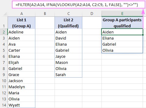
6.2. Using the FILTER Function (Excel 365 and Excel 2021):

The FILTER function provides a dynamic way to extract the common values directly into a new range, without the need for manual filtering.

Syntax:

=FILTER(array, include, [if_empty])

• array: The range of cells you want to filter (List 1 in this case).
• include: A logical array (TRUE/FALSE values) that determines which rows to include in the result.
• [if_empty]: Optional. The value to return if the filter results in an empty array.

Formula:

=FILTER(A2:A14, IFNA(VLOOKUP(A2:A14, C2:C9, 1, FALSE), "")<>"")

Explanation:

1. A2:A14: This is the array argument, representing List 1 (the list of participants).
2. IFNA(VLOOKUP(A2:A14, C2:C9, 1, FALSE), “”)<>””: This is the include argument. Let’s break it down further:
   • VLOOKUP(A2:A14, C2:C9, 1, FALSE): This performs the VLOOKUP for each value in List 1, searching for it in List 2. It returns an array of matches and #N/A errors.
   • IFNA(…, “”): This replaces the #N/A errors with empty strings, resulting in an array of matches and empty strings.
   • <>””: This compares each element in the array to an empty string. It returns TRUE for matches (because they are not equal to an empty string) and FALSE for empty strings (because they are equal to an empty string).

In essence, the FILTER function uses the include argument to select only the rows from List 1 where the corresponding VLOOKUP result is a match (i.e., not an empty string).

Alternative with ISNA:

You can also use the ISNA function to achieve the same result:

=FILTER(A2:A14, ISNA(VLOOKUP(A2:A14, C2:C9, 1, FALSE))=FALSE)

This formula filters List 1 based on whether the VLOOKUP result is not a #N/A error (i.e., a match was found).

Using XLOOKUP:

If you are using Excel 365 or Excel 2021, you can simplify the formula even further using the XLOOKUP function:

=FILTER(A2:A14, XLOOKUP(A2:A14, C2:C9, C2:C9,"")<>"")

7. Finding Missing Values (Differences) Between Two Columns

To identify values that exist in one column but not the other, you can modify the VLOOKUP formula to specifically look for the #N/A errors (or their replacements).

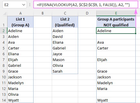
7.1. Using IF and ISNA:

=IF(ISNA(VLOOKUP(A2, $C$2:$C$9, 1, FALSE)), A2, "")

Explanation:

1. VLOOKUP(A2, $C$2:$C$9, 1, FALSE): Performs the basic VLOOKUP to search for the value in A2 within List 2.
2. ISNA(…): Checks if the VLOOKUP result is a #N/A error. Returns TRUE if it is, and FALSE if it isn’t.
3. IF(ISNA(…), A2, “”):
   • If ISNA returns TRUE (meaning the value is not found in List 2), the IF function returns the value from A2 (the missing value).
   • If ISNA returns FALSE (meaning the value is found in List 2), the IF function returns an empty string.

This formula will give you a list where missing values from List 1 are displayed, and matches are represented by blank cells. You can then use AutoFilter to remove the blanks and get a clean list of differences.

7.2. Using the FILTER Function (Excel 365 and Excel 2021):

For a dynamic solution, use the FILTER function in combination with ISNA:

=FILTER(A2:A14, ISNA(VLOOKUP(A2:A14, C2:C9, 1, FALSE)))

This formula directly filters List 1, including only the values for which the ISNA(VLOOKUP(...)) condition is TRUE (i.e., the values that are not found in List 2).

Alternative with XLOOKUP:

=FILTER(A2:A14, XLOOKUP(A2:A14, C2:C9, C2:C9,"")="")

8. Identifying Matches and Differences with Text Labels

Instead of just returning matches or differences, you can use VLOOKUP to add text labels to your data, indicating whether each value is present in both lists or only in one.

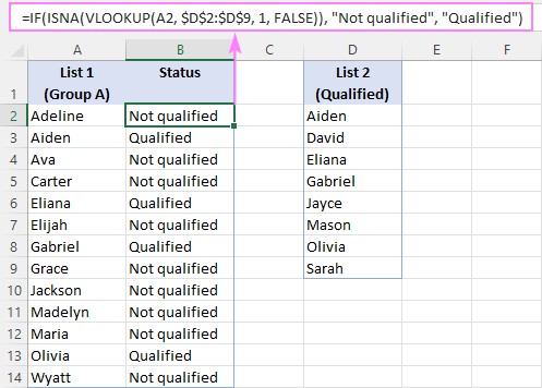
8.1. The Formula:

=IF(ISNA(VLOOKUP(A2, $D$2:$D$9, 1, FALSE)), "Not in List 2", "In List 2")

Explanation:

This formula builds upon the previous examples by incorporating the IF function to assign text labels based on whether a match is found.

1. VLOOKUP(A2, $D$2:$D$9, 1, FALSE): Performs the standard VLOOKUP.
2. ISNA(…): Checks for #N/A errors.
3. IF(ISNA(…), “Not in List 2”, “In List 2”):
   • If ISNA returns TRUE (value not found), the formula returns “Not in List 2”.
   • If ISNA returns FALSE (value found), the formula returns “In List 2”.

You can customize the text labels to suit your specific needs. For example:

=IF(ISNA(VLOOKUP(A2, $D$2:$D$9, 1, FALSE)), "Not Qualified", "Qualified")

8.2. Using the MATCH Function:

The MATCH function can also be used to achieve the same result:

=IF(ISNA(MATCH(A2, $D$2:$D$9, 0)), "Not in List 2", "In List 2")

The MATCH function returns the position of a value within a range. If the value is not found, it returns a #N/A error. The rest of the formula works the same way as the VLOOKUP version.

9. Returning a Value from a Third Column Based on a Match

One of the most common uses of VLOOKUP is to retrieve related information from another column based on a match between two columns.

9.1. Scenario:

You have two tables:

• Table 1 (Columns A & B): Contains a list of names (Column A) and their corresponding IDs (Column B).
• Table 2 (Columns D & E): Contains a list of names (Column D) and their scores (Column E).

You want to add the scores from Table 2 to Table 1, based on the matching names.

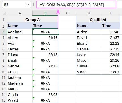
9.2. The Formula:

=VLOOKUP(A2, $D$2:$E$10, 2, FALSE)

Explanation:

1. A2: The lookup value (the name from Table 1).
2. $D$2:$E$10: The table array (Table 2, including both the names and the scores).
3. 2: The column index number. Since the scores are in the second column of Table 2, we use 2.
4. FALSE: We want an exact match.

This formula will search for the name in A2 within Column D of Table 2. If a match is found, it will return the corresponding score from Column E (the second column of the table array).

9.3. Handling Missing Values:

Use IFNA or IFERROR to handle cases where a name in Table 1 is not found in Table 2:

=IFNA(VLOOKUP(A2, $D$2:$E$10, 2, FALSE), "Not Available")

This will return “Not Available” if a matching score is not found.

9.4. Alternative with INDEX and MATCH:

The INDEX and MATCH functions provide a more flexible alternative to VLOOKUP:

=IFNA(INDEX($E$2:$E$10, MATCH(A2, $D$2:$D$10, 0)), "Not Available")

Explanation:

1. MATCH(A2, $D$2:$D$10, 0): Finds the row number where the name in A2 is located in Column D of Table 2.
2. INDEX($E$2:$E$10, …): Returns the value from Column E (the scores) at the row number returned by the MATCH function.

9.5. Alternative with XLOOKUP:

=XLOOKUP(A2, $D$2:$D$10, $E$2:$E$10, "Not Available")

10. VLOOKUP vs. Other Comparison Methods

While VLOOKUP is a powerful tool for comparing columns, it’s not always the best solution. Here’s a brief comparison to other methods:

Method	Strengths	Weaknesses	Use Cases
VLOOKUP	Simple, widely understood, good for returning related data	Only searches in the first column, can be inefficient for large datasets, error-prone	Finding matches, returning corresponding values, simple comparisons
MATCH & INDEX	More flexible than VLOOKUP, can search in any column	More complex syntax	Finding matches and returning values when the lookup column is not the first column
XLOOKUP	Modern, more flexible, handles errors better, can search in any direction	Only available in Excel 365 and Excel 2021	General-purpose lookup and comparison, replacing VLOOKUP and INDEX/MATCH
COUNTIF	Simple for checking if a value exists	Doesn’t return related data, can be slow for large datasets	Checking for the existence of a value, counting occurrences
Conditional Formatting	Visually highlights matches or differences	Doesn’t create a separate list of matches/differences	Quickly identifying matches or differences in place, visual analysis
Power Query	Powerful for data cleaning, transformation, and comparison	Steeper learning curve, requires understanding of Power Query concepts	Complex data manipulation, combining data from multiple sources, handling large datasets

11. Best Practices for Using VLOOKUP to Compare Columns

• Use absolute references ($) for the table_array: This ensures that the range remains fixed when you copy the formula.
• Use IFNA or IFERROR to handle #N/A errors: This improves the readability of your results and prevents errors from propagating through your calculations.
• Consider using XLOOKUP if you have Excel 365 or Excel 2021: It’s more flexible and easier to use than VLOOKUP.
• Be aware of the limitations of VLOOKUP: It only searches in the first column of the table_array and can be inefficient for large datasets.
• Choose the right comparison method for your specific needs: VLOOKUP is not always the best solution. Consider other methods like MATCH, INDEX, XLOOKUP, COUNTIF, conditional formatting, or Power Query.
• Ensure data types are consistent: VLOOKUP requires that the data types of the lookup_value and the values in the first column of the table_array are the same.
• Sort data when using approximate match (range_lookup = TRUE): VLOOKUP with approximate match requires that the first column of the table_array is sorted in ascending order.
• Test your formulas thoroughly: Before relying on the results of your VLOOKUP formulas, make sure to test them with a variety of data to ensure that they are working correctly.

12. VLOOKUP and Data Integrity

When using VLOOKUP to compare columns, maintaining data integrity is crucial for accurate results. Here are some key considerations:

12.1. Data Type Consistency:

Ensure that the data types in your lookup column and the first column of your table array are consistent. For example, if you’re comparing numbers, make sure both columns are formatted as numbers and not text. Inconsistent data types can lead to VLOOKUP not finding matches even when they exist.

12.2. Handling of Case Sensitivity:

VLOOKUP is not case-sensitive. This means “Apple” and “apple” will be considered a match. If you need case-sensitive comparisons, you’ll need to use more complex formulas involving the EXACT function.

12.3. Dealing with Leading and Trailing Spaces:

Leading and trailing spaces can also cause VLOOKUP to fail to find matches. Use the TRIM function to remove these spaces from your data before performing the VLOOKUP.

12.4. Consistent Formatting:

Ensure that the formatting of your data is consistent. This includes things like date formats, currency symbols, and decimal places. Inconsistent formatting can lead to VLOOKUP not finding matches even when the underlying values are the same.

12.5. Error Checking and Validation:

Implement error checking and validation to ensure that your data is accurate and consistent. This can include using data validation rules to restrict the types of data that can be entered into a cell, as well as using formulas to check for errors and inconsistencies.

13. Advanced Techniques and Considerations

13.1. Using VLOOKUP with Wildcards:

VLOOKUP can be used with wildcards to perform partial matches. The wildcard characters are:

• *: Matches any sequence of characters.
• ?: Matches any single character.

For example, to find a value that starts with “App”, you can use the following formula:

=VLOOKUP("App*", $A$1:$B$10, 2, FALSE)

13.2. VLOOKUP with Multiple Criteria:

VLOOKUP can only search based on a single criterion. To search based on multiple criteria, you can create a helper column that concatenates the values of the multiple criteria into a single string. Then, you can use VLOOKUP to search for the concatenated string.

13.3. VLOOKUP for Approximate Matching:

When the range_lookup argument is set to TRUE, VLOOKUP performs an approximate match. This means that if VLOOKUP cannot find an exact match, it will return the next largest value that is less than the lookup value. Approximate matching can be useful for looking up values in a table that contains ranges of values.

13.4. Limitations of VLOOKUP and Alternatives:

VLOOKUP has several limitations:

• It can only search in the first column of the table array.
• It is not case-sensitive.
• It can be inefficient for large datasets.

Alternatives to VLOOKUP include:

• INDEX and MATCH: These functions can be used together to perform more flexible lookups.
• XLOOKUP: This is a newer function that is more flexible and easier to use than VLOOKUP.
• Power Query: This is a powerful tool for data cleaning, transformation, and analysis.

14. Real-World Examples and Use Cases

14.1. Inventory Management:

Compare a list of products sold with a list of products in stock to identify items that need to be reordered. Use VLOOKUP to find the quantity in stock for each item sold and flag items below a certain threshold.

14.2. Customer Relationship Management (CRM):

Compare a list of new leads with a list of existing customers to identify potential duplicates. Use VLOOKUP to find existing customer records based on email address or phone number and merge information.

14.3. Financial Analysis:

Compare a list of transactions with a budget to identify variances. Use VLOOKUP to find the budgeted amount for each transaction category and calculate the difference.

14.4. Human Resources:

Compare a list of employees with a list of training courses completed to identify employees who need additional training. Use VLOOKUP to find the training courses completed by each employee and identify gaps.

14.5. Sales and Marketing:

Compare a list of marketing leads with a list of sales opportunities to identify potential conversions. Use VLOOKUP to find the sales opportunity associated with each marketing lead and track conversion rates.

15. VLOOKUP Troubleshooting: Common Errors and Solutions

15.1. #N/A Error:

• Cause: VLOOKUP cannot find the lookup_value in the first column of the table_array.
• Solution:
  • Verify that the lookup_value exists in the first column of the table_array.
  • Check for spelling errors, leading/trailing spaces, and inconsistent data types.
  • Ensure that the range_lookup argument is set correctly (FALSE for exact match, TRUE for approximate match).
  • If using approximate match, make sure the first column of the table_array is sorted in ascending order.

15.2. #REF! Error:

• Cause: The col_index_num argument is greater than the number of columns in the table_array.
• Solution:
  • Verify that the col_index_num argument is within the range of columns in the table_array.

15.3. Incorrect Results:

• Cause: VLOOKUP is returning the wrong value.
• Solution:
  • Verify that the table_array argument is correct and includes all the necessary data.
  • Check that the col_index_num argument is pointing to the correct column.
  • Ensure that the range_lookup argument is set correctly (FALSE for exact match, TRUE for approximate match).
  • If using approximate match, make sure the first column of the table_array is sorted in ascending order.

15.4. Performance Issues:

• Cause: VLOOKUP is slow for large datasets.
• Solution:
  • Consider using alternative methods like INDEX and MATCH, XLOOKUP, or Power Query.
  • Optimize your data by removing unnecessary columns and rows.
  • Ensure that your data is properly indexed.

16. The Future of Excel and Data Comparison

Excel continues to evolve, with Microsoft regularly adding new features and functions. Functions like XLOOKUP represent a significant improvement over VLOOKUP, offering greater flexibility and ease of use. AI-powered features are also being integrated into Excel, promising to automate and simplify data analysis tasks.

Other data comparison tools, such as specialized data comparison software and cloud-based platforms, are also becoming increasingly popular. These tools often offer more advanced features and capabilities than Excel, such as the ability to compare data from different sources, perform complex data transformations, and generate detailed reports.

Despite these advancements, Excel remains a valuable tool for data comparison, especially for users who are already familiar with its interface and functionality. By mastering techniques like VLOOKUP and staying up-to-date with the latest Excel features, users can continue to leverage Excel for their data comparison needs.

17. Conclusion: Mastering VLOOKUP for Excel Column Comparison

VLOOKUP is a versatile Excel function that empowers you to compare columns, identify matches and differences, and retrieve related data. By understanding its syntax, mastering error handling, and exploring advanced techniques, you can significantly enhance your data analysis skills.

Remember to choose the right comparison method for your specific needs and always prioritize data integrity. As Excel continues to evolve, staying updated with new features and best practices will ensure you can effectively leverage this powerful tool for all your data comparison tasks.

Ready to take your Excel skills to the next level? Visit COMPARE.EDU.VN today to discover more comprehensive guides, tutorials, and resources to help you master Excel and other essential software tools. Make informed decisions with confidence – COMPARE.EDU.VN is your trusted source for objective comparisons and expert insights.

Address: 333 Comparison Plaza, Choice City, CA 90210, United States

Whatsapp: +1 (626) 555-9090

Website: compare.edu.vn

18. Frequently Asked Questions (FAQ) About Comparing Excel Columns with VLOOKUP

1. Can VLOOKUP compare columns in two different Excel files?

Yes, VLOOKUP can compare columns in different Excel files. You need to use the full path to the external file in the table_array argument. For example: '[FileName.xlsx]SheetName'!$A$1:$B$10. However, both files need to be open for the formula to work correctly.

2. How do I make VLOOKUP case-sensitive?

VLOOKUP is not case-sensitive. To perform a case-sensitive lookup, you can use a combination of INDEX, MATCH, and EXACT functions. This involves using EXACT to compare the case and MATCH to find the position, then INDEX to return the corresponding value.

3. What does the #N/A error mean in VLOOKUP?

The #N/A error in VLOOKUP means that the function could not find the lookup_value in the first column of the table_array. This could be due to a spelling error, incorrect data type, or the value simply not existing in the lookup range.

4. Can I use VLOOKUP to return multiple values?

VLOOKUP is designed to return a single value from a specified column. To return multiple values, you would need to use multiple VLOOKUP formulas, each with a different col_index_num to return a different column’s value. Alternatively, consider using INDEX and MATCH or XLOOKUP, which can be more flexible.

5. How can I improve VLOOKUP performance with large datasets?

VLOOKUP can be slow with large datasets. To improve performance:

• Ensure the lookup column is indexed.
• Use XLOOKUP if available.
• Consider using Power Query for more complex data transformations and comparisons.
• Avoid using VLOOKUP on entire columns (e.g., A:A), and instead, use specific ranges (e.g., A1:A1000).

6. Is there a limit to the number of rows VLOOKUP can handle?

Excel has a limit to the number of rows and columns in a worksheet, which indirectly affects VLOOKUP. As of Excel 2016, a worksheet can contain 1,048,576 rows and 16,384 columns. VLOOKUP can operate on any range within these limits, but performance may degrade with very large datasets.

7. How do I prevent VLOOKUP from returning errors when there’s no match?

You can prevent VLOOKUP from returning errors by wrapping it in an IFERROR or IFNA function. This allows you to specify a value to return when VLOOKUP does not find a match, such as an empty string (“”), “Not Found”, or any other custom text.

8. Can VLOOKUP search for values in multiple columns?

No, VLOOKUP can only search for values in the first column of the table_array. To search in multiple columns, you would need to create a helper column that concatenates the values from those columns and then use VLOOKUP on the helper column.

9. How does VLOOKUP handle duplicate values in the lookup column?

VLOOKUP will return the first match it finds when there are duplicate values in the lookup column. If you need to handle duplicates differently (e.g., return all matches), you’ll need to use more advanced techniques involving array formulas or Power Query.

10. What are the best alternatives to VLOOKUP in Excel?

The best alternatives to VLOOK