How To Compare Two Excel Columns To Find Matches effectively? COMPARE.EDU.VN simplifies the process of identifying similarities between data sets. Discover proven techniques and tools to streamline your comparisons, ensuring accuracy and saving you time. Explore methods for data matching, duplicate detection, and data validation, ultimately leading to improved data analysis and informed decision-making with enhanced spreadsheet proficiency.
1. Why Is Comparing Two Columns in Excel Important?
Excel is essential for storing data, performing calculations, and making informed decisions. It’s a versatile tool that helps users understand and present information effectively. Data analysts rely on Excel to gather insights crucial for marketing and sales strategies. When cells lack information, depending on the formulas or tools used, it can significantly impact the results. Because spreadsheets often contain large amounts of data and are interconnected, data analysts frequently need to compare columns within the same or different spreadsheets. Manually comparing these columns can be a time-consuming and error-prone task, potentially taking hours or even days to locate missing data.
Comparing two columns in Excel is vital for data analysts to determine whether a cell contains data or not. Excel simplifies this process by displaying results as TRUE/FALSE, Match/Not Match, or any other user-defined message, making it easier to identify and address discrepancies.
2. What Are the Different Methods To Compare Two Columns in Excel?
When working with data in multiple columns, tables, or spreadsheets, it is often necessary to compare them to identify data that is either missing or present in both. Comparisons can be approached in several ways, and the choice of method depends on the specific requirements of the task. Here are some common methods for comparing two columns in Excel:
- Highlighting Unique or Duplicate Values: Employ functions or conditional formatting to emphasize values that are either unique or duplicated across the columns.
- Displaying Unique or Duplicate Values: Utilize conditional formatting or formulas to distinctly show unique or duplicate entries.
- Row-by-Row Comparison: Conduct a direct comparison of each row to find matching data.
- Using LOOKUP Formulas: Apply LOOKUP functions to search for specific values and identify matches or differences.
3. How To Compare Two Columns in Excel Using The Equals Operator?
You can compare two columns row by row to find matching data, returning results like Match or Not Match. For instance, the formula =A2=B2 can determine matching data, displaying True or False.
Enter the formula into cell C2 and drag it down the column. The formula returns TRUE if the values in the compared rows are identical and FALSE otherwise.
4. How To Compare Two Excel Columns With The IF Condition?
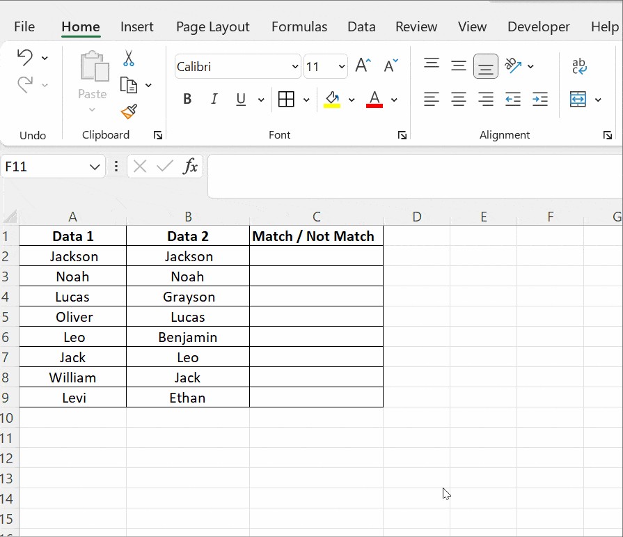
In Excel, using an IF condition to compare two columns is a straightforward process. The formula =IF(A2=B2,”Match”,” “) returns “Match” for rows with identical values, leaving the remaining rows blank.
The same formula can identify and highlight differing values by displaying a specific result when the IF condition is false. To achieve this, use the formula =IF(A2=B2,”Match”,”Not a Match”).
To compare two columns and identify differences, substitute the equals sign with a non-equality sign (). The formula is =IF(A2B2,”Match”,”Not a Match”).
5. How To Compare Two Excel Columns Using The EXACT() Function?
When comparing two columns in Excel, use the EXACT() function to find case-sensitive values.
The EXACT() function compares two text strings and returns TRUE if they are identical and FALSE otherwise. EXACT is case-sensitive but ignores formatting differences. The syntax is =EXACT(text1, text2), where both text1 and text2 are required arguments.
Consider a simple example where columns data1 and data2 contain the text string “Nova Scotia” in columns A and B.
Applying the formula =IF(A2=B2, “Match”, “Mismatch”) to cell C2 returns a match because it is case-insensitive.
Use the formula =IF(EXACT(A2, B2), “Match”, “Mismatch”) for the IF condition to be case-sensitive.
The EXACT() function returns values as true or false. The function works by executing the inner function first and then returning the result. In the above example, the EXACT() function returns a false value to the outer function IF.
The IF condition generally works such that if it returns true, the first argument in the function is returned; otherwise, the second argument is returned.
6. How To Use Conditional Formatting To Compare Two Columns in Excel?
To use conditional formatting, first, click Home, then Styles, and follow these steps: Conditional Formatting → Highlight Cell Rules → Duplicate Values. A dialogue box will appear, as shown below, allowing you to select values from the drop-down menu.
Apply the formatting condition to the cells. You can choose from various conditions, such as Duplicate or Unique, and then select options like filling with color, changing the text color, or altering the cell border.
In the example below, there are two datasets with names listed in the Data1 and Data2 columns. Not all names from Data1 are in Data2. To find and highlight names present in both columns, use Conditional Formatting.
Before applying Conditional Formatting, select the entire table and follow the steps mentioned above. Choose Duplicate to find names in both columns. Then, select an option to highlight the duplicates, such as filling the cells with color, changing the text color, or modifying the cell border.
The Custom Format option allows you to highlight cells with a color of your choice, beyond the options available in the drop-down menu.
Another useful option is Unique. Select this if you want to highlight cells containing data that is not repeated, effectively highlighting unique entries.
Instead of selecting Duplicate, choose Unique from the drop-down list and apply a highlighting option, such as filling with color, changing the text color, or changing the cell border.
Tip: To remove formatting from cells, go to Conditional Formatting → Clear Rules → Clear Rules from Selected Cells.
Use conditional formatting when you don’t need a third column to display comparison results. Here, you can highlight duplicate (matching) and unique (different) data to show which rows have the same data or use an additional column to display values indicating whether the data matches. These methods are best suited for smaller tables, as large spreadsheets require more complex approaches.
This is an effective way to compare two columns in Excel and identify differences.
7. How To Use The LOOKUP Function To Compare Two Columns in Excel?
The LOOKUP function is designed to find a specific value in a single row or column and then return a corresponding value from another row or column. There are several types of lookup functions available, including HLOOKUP, VLOOKUP, and XLOOKUP. The letters H and V stand for horizontal and vertical, respectively. The XLOOKUP function combines the capabilities of both LOOKUP and VLOOKUP.
The example below demonstrates how to compare two columns in Excel to identify differences using the VLOOKUP() function.
Column A contains a list of exams taken by a student, and column B lists the subjects the student passed. The result sheet should include a list of all subjects. The VLOOKUP() is applied in cell C2 as =VLOOKUP(A2, $B$2:$B$5,1,0).
Drag the formula down to apply it to all cells below C2. The result in column C indicates which subjects were cleared and which were not, marked as #N/A. The VLOOKUP formula in Excel to compare two columns is as follows:
- VLOOKUP(A2,..,..,..) – retrieves the value in cell A2.
- VLOOKUP(A2, $B$2:$B$5,..,..) – compares the value from A2 with all values in the range B2 to B5. The cells in the range B2:B5 are locked using absolute references, indicated by the $ symbol.
- VLOOKUP(A2, $B$2:$B$5,1,..) – the third argument, col_index_num, specifies the column to compare from the lookup value A2. In this example, the subjects are listed in column A, and the comparison column is one column away. Hence, the value is 1.
- VLOOKUP(A2, $B$2:$B$5,1,0) – the last argument takes a logical value, either 0 or 1. Use 0 (zero) to find an exact match. Use 1 to have VLOOKUP() return the closest match sorted in ascending order.
8. How To Use The Find & Select Option To Compare Two Columns in Excel?
Comparing two columns using the “Find & Select” option in Excel is a quick method to highlight differences. Here’s how you can do it:
-
Select the Columns: Start by selecting the two columns you want to compare. Click on the column headers (e.g., A and B) to select the entire columns.
-
Open Go To Special: Go to the Home tab on the Excel ribbon. In the Editing group, click on Find & Select, and then choose Go To Special… from the dropdown menu.
-
Choose Row Differences: In the Go To Special dialog box, select Row differences. This option tells Excel to find cells that differ between the selected columns on each row.
-
Click OK: After selecting Row differences, click OK. Excel will select only the cells that are different between the two columns.
-
Highlight the Differences: Now that the differing cells are selected, you can highlight them to make the differences visually clear. In the Home tab, go to the Font group and use the Fill Color tool to choose a color. Click the color to highlight the selected cells.
9. What Are Some Practical Applications of Comparing Two Columns?
Comparing two columns in Excel is a versatile technique with numerous practical applications across various fields. Here are some key scenarios where this method proves invaluable:
- Data Validation: Ensuring data accuracy by comparing entries in two columns to identify discrepancies. This is particularly useful when cross-referencing data from different sources or verifying data entry accuracy.
- Duplicate Detection: Identifying duplicate entries within a dataset by comparing a column against itself or another column containing similar data. This helps in cleaning up databases and avoiding redundant information.
- Change Tracking: Monitoring changes in a dataset over time by comparing two versions of the same column. This is useful for tracking updates, additions, or deletions in a list or database.
- List Reconciliation: Matching items between two lists to ensure completeness and accuracy. For example, comparing a list of customers against a list of sales transactions to identify missing entries.
- Database Management: Comparing columns in two different tables to find related data or identify inconsistencies. This is essential for maintaining data integrity and ensuring that databases are properly linked.
- Inventory Management: Comparing stock levels recorded in two different systems to reconcile discrepancies and ensure accurate inventory tracking.
- Financial Auditing: Comparing financial records from different sources to detect errors or fraud. This can involve comparing transaction logs, invoices, and bank statements.
- Research Analysis: Comparing experimental data from two different groups or conditions to identify significant differences. This is common in scientific research and statistical analysis.
- Merging Data: Identifying common entries between two columns before merging them into a single, unified dataset. This helps avoid duplication and ensures that the merged data is accurate and complete.
10. Frequently Asked Questions
10.1 How to compare two columns in Excel to find differences?
To compare two columns in Excel to find differences, select both columns, then go to Home → Find & Select → Go To Special → Row Differences, and click OK. The matching cells will appear white, while the unmatched cells will be gray.
10.2 What are alternative methods for comparing two columns in Excel using the IF condition?
To find matches in all cells within the same row in a table with three or more columns, use an IF formula with an AND statement: =IF(AND(A2=B2, A2=C2), “Full match”, “”). To find matches in any two cells in the same row, use: =IF(OR(A2=B2, B2=C2, A2=C2), “Match”, “”).
10.3 Can you compare two columns in Excel using the Index-Match function?
Yes, you can use the INDEX-MATCH function to compare two columns in different tables and pull matching entries. The MATCH() function compares values from one column to another, and if a match is found, it pulls the corresponding value from another column; otherwise, it returns #N/A.
For example: INDEX(B2:B4,MATCH(D2,A2:A4,0)). In this formula, the MATCH() function takes all the values in column D starting from D2 and compares them with those in column A from A2 to A4. If it finds a match, it pulls the corresponding value from column B and displays it; otherwise, it returns a value #N/A.
Conclusion
We often need to compare columns in Excel. Microsoft Excel offers options to compare and match data in single columns, multiple columns, and multiple spreadsheets. This tutorial shows you several methods to compare two columns for matches in Excel.
LOOKUP() functions are vital to learn in Excel as they’re so widely used. Take a look at VLOOKUP in-depth tutorial, and you can work with other lookup functions (HLOOKUP and XLOOKUP), too.
For more in-depth knowledge of Excel functions and formulas, consider exploring courses on our website, COMPARE.EDU.VN.
Ready to make data comparisons easier? Visit compare.edu.vn today to discover our comprehensive comparison tools and resources. Make informed decisions with confidence. Contact us at 333 Comparison Plaza, Choice City, CA 90210, United States, or via Whatsapp at +1 (626) 555-9090.
