Comparing two Excel columns to find duplicates is a common task. COMPARE.EDU.VN provides a comprehensive guide to help you achieve this efficiently. By using formulas and features within Excel, you can quickly identify duplicate entries, ensuring data accuracy and saving valuable time. This process involves using techniques like conditional formatting, the equals operator, and functions like VLOOKUP and EXACT to highlight and manage duplicate data, enhancing data integrity and analysis. Explore data comparison, data matching, and duplicate identification using Excel.
1. Understanding the Need to Compare Excel Columns for Duplicates
Data analysis often requires comparing columns to find duplicate entries. This is crucial for maintaining data integrity and accuracy. Finding duplicates in Excel columns is essential for data cleaning, reporting, and decision-making. Manual comparison can be time-consuming and prone to errors, especially with large datasets. Therefore, effective methods for identifying and managing duplicates are essential.
2. Why is Finding Duplicates Important?
Identifying duplicates helps in several ways:
- Data Cleaning: Removes redundant information.
- Accuracy: Ensures data is accurate and reliable.
- Efficiency: Speeds up data processing and analysis.
- Decision Making: Improves the quality of insights derived from the data.
According to a study by the Technology University of Munich, data quality issues, including duplicates, can lead to a 15-25% reduction in revenue for organizations.
3. Methods for Comparing Two Excel Columns
There are several methods to compare two Excel columns to find duplicates, each with its advantages.
- Conditional Formatting
- Equals Operator
- VLOOKUP Function
- IF Formula
- EXACT Formula
3.1. Using Conditional Formatting
Conditional formatting is a straightforward method to highlight duplicates.
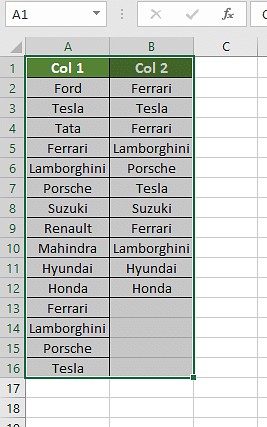
Step 1: Select the Columns
Select the two columns you want to compare.
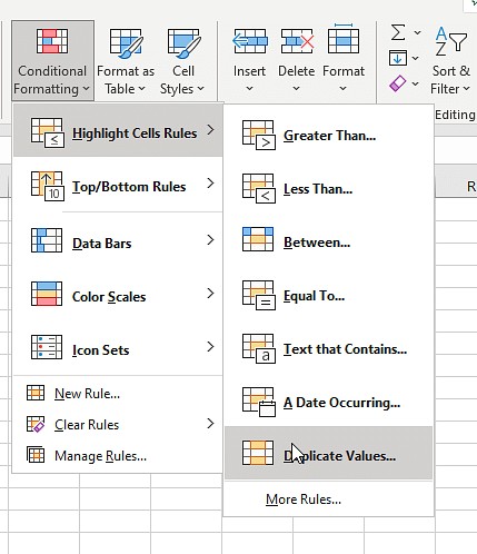
Step 2: Access Conditional Formatting
Go to the “Home” tab, click “Conditional Formatting,” and choose “Highlight Cells Rules,” then “Duplicate Values.”
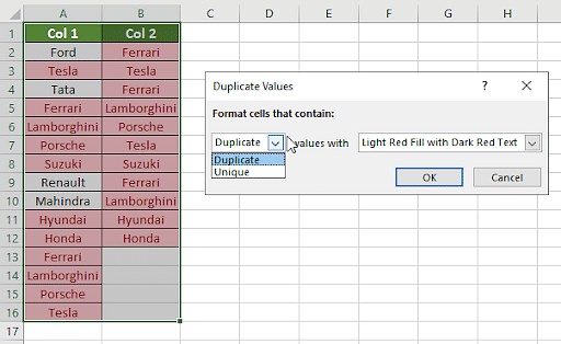
Step 3: Choose Formatting Options
Select the formatting style for duplicate values and click “OK.” Excel will highlight all duplicate entries in the selected columns.
A. Duplicate Values
This option highlights matching values between the two columns, useful for identifying identical data points.
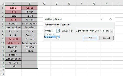
B. Unique Values
Alternatively, you can highlight unique values to identify entries that appear only once in the selected columns.
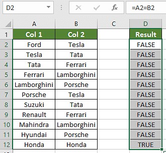
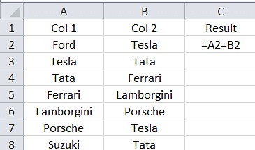
3.2. Using the Equals Operator
The equals operator (=) allows for a cell-by-cell comparison.
Step 1: Create a Result Column
Create a new column next to the columns you are comparing.
Step 2: Enter the Formula
In the first cell of the result column, enter the formula =A1=B1, where A1 and B1 are the first cells in your columns.
Step 3: Apply the Formula
Drag the formula down to apply it to all rows. Excel will display “TRUE” for matching cells and “FALSE” for non-matching cells.
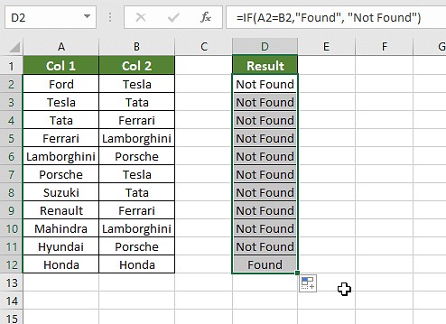
Step 4: Customize with IF Clause
To display custom messages, use the IF clause. For example, =IF(A1=B1, "Match", "No Match").
The final result will display “Match” or “No Match” based on whether the values in the compared cells are the same.
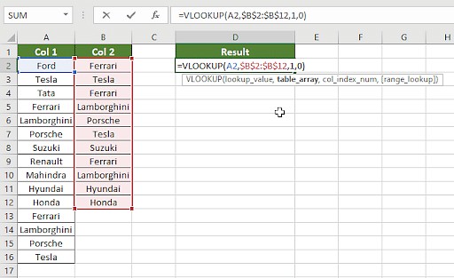
3.3. Using the VLOOKUP Function
The VLOOKUP function is useful for finding matches between columns.
Step 1: Create a Result Column
Create a new column next to the columns you are comparing.
Step 2: Enter the VLOOKUP Formula
In the first cell of the result column, enter the VLOOKUP formula:
=VLOOKUP(A1,B:B,1,FALSE)
Here, A1 is the lookup value (the first cell in column A), B:B is the table array (column B), 1 is the column index number (since we are looking in one column), and FALSE ensures an exact match.
Step 3: Apply the Formula
Drag the formula down to apply it to all rows.
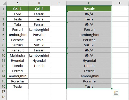
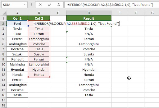
Step 4: Handle Errors
To avoid errors for non-matching values, use the IFERROR clause. For example:
=IFERROR(VLOOKUP(A1,B:B,1,FALSE), "Not Found")
This will display “Not Found” for values in column A that do not exist in column B.
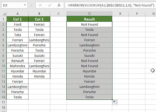
Step 5: Final Error-Free Result
The final result will show the matching values or “Not Found” for each entry.
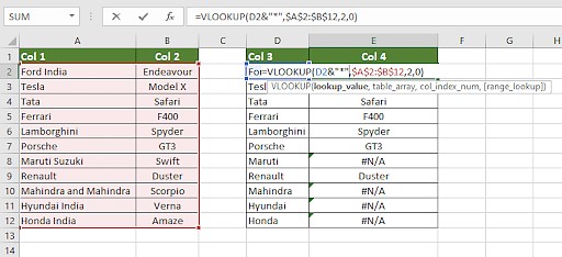
Step 6: Using Wildcards for Partial Matches
In real-world scenarios, data might vary slightly. For example, one column might have “Ford India” while the other has “Ford.” To handle this, use wildcards.
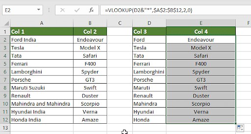
Step 7: Modified Formula with Wildcards
Modify the formula to include wildcards:
=IFERROR(VLOOKUP(A1&"*",B:B,1,FALSE), "Not Found")
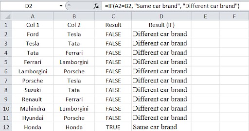
3.4. Using the IF Formula
The IF formula is used to display a desired result for a similarity or a difference.
Step 1: Enter the IF Formula
Enter the IF formula in the result column:
=IF(A2=B2,"Match","Different")
This formula compares the values in cells A2 and B2. If they match, it returns “Match”; otherwise, it returns “Different.”
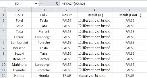
3.5. Using the EXACT Formula
The EXACT formula compares two strings and returns TRUE if they are exactly the same, including case.
Step 1: Enter the EXACT Formula
Enter the EXACT formula in the result column:
=EXACT(A2, B2)
If the value in one column is exactly the same as the other column, the result will be displayed as “TRUE,” and if the values are not equal, the result will be “FALSE.”
The EXACT formula is case-sensitive, so “Honda” and “honda” will be considered different.
4. Choosing the Right Comparison Method
Selecting the appropriate method depends on the specific scenario.
4.1. Comparing Row-by-Row
To compare two columns row-by-row, use the IF or EXACT formulas.
=IF(A2 = B2, "Match", " ")=IF(A2<>B2, "No match", " ")=IF(EXACT(A2, B2), "Match", " ")(for case-sensitive comparison)
4.2. Comparing Multiple Columns
For comparing multiple columns, use the AND or COUNTIF functions.
=IF(AND(A2=B2, A2=C2), "Complete match", " ")=IF(COUNTIF($A2:$E2, $A2)=4, "Complete match", " ")(where 4 is the number of columns being compared)
4.3. Finding Matches and Differences
To find unique values in one column compared to another, use the COUNTIF or MATCH functions.
=IF(COUNTIF($B:$B, $A2)=0, "Not present in B", " ")=IF(ISERROR(MATCH($A2,$B$2:$B$10,0)),"Not present in B","")
4.4. Comparing Lists and Pulling Matching Data
To compare two lists and find matching data, use the VLOOKUP or INDEX MATCH functions.
=VLOOKUP(D2, $A$2:$B$6, 2, FALSE)=INDEX($B$2:$B$6, MATCH($D2, $A$2:$A$6, 0))=XLOOKUP(D2, $A$2:$A$6, $B$2:$B$6)
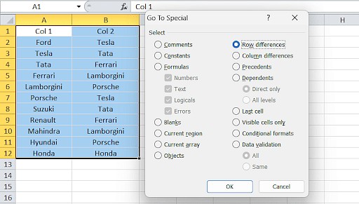
4.5. Highlighting Row Matches and Differences
Use conditional formatting with formulas to highlight rows with matches or differences.
=AND($A2=$B2, $A2=$C2)=COUNTIF($A2:$C2, $A2)=3(where 3 is the number of columns)
Additionally, use the “Go To Special” feature to highlight row differences.
5. Common Scenarios and Solutions
Here are a few common scenarios and how to address them:
| Scenario | Method | Formula/Steps |
|---|---|---|
| Find Duplicates | Conditional Formatting | Home > Conditional Formatting > Highlight Cells Rules > Duplicate Values |
| Cell-by-Cell Comparison | Equals Operator | =A1=B1 |
| Find Matches in Another Column | VLOOKUP | =VLOOKUP(A1,B:B,1,FALSE) |
| Custom Match/No Match Results | IF Formula | =IF(A2=B2,"Match","No Match") |
| Case-Sensitive Comparison | EXACT Formula | =EXACT(A2, B2) |
| Partial Matches | VLOOKUP with Wildcards | =IFERROR(VLOOKUP(A1&"*",B:B,1,FALSE), "Not Found") |
| Highlight Row Differences | Conditional Formatting & “Go To Special” | 1. Select Columns 2. Home > Find & Select > Go To Special > Row Differences 3. Apply Formatting to Highlight |
| Compare Two Lists | VLOOKUP, INDEX MATCH, or XLOOKUP | =VLOOKUP(D2, $A$2:$B$6, 2, FALSE), =INDEX($B$2:$B$6, MATCH($D2, $A$2:$A$6, 0)), =XLOOKUP(D2, $A$2:$A$6, $B$2:$B$6) |
6. Advanced Techniques
- Using Array Formulas: For more complex comparisons, array formulas can be employed to compare entire ranges at once.
- Combining Functions: Combine multiple functions like IF, AND, OR, and COUNTIF for advanced logical comparisons.
- Power Query: Use Power Query for advanced data transformation and comparison tasks.
7. Tips for Efficient Comparison
- Sort Data: Sort columns to group similar values together, making visual inspection easier.
- Use Filters: Apply filters to display only matching or non-matching values.
- Automate Tasks: Use VBA scripts to automate repetitive comparison tasks. According to research by the University of Pennsylvania’s Wharton School, automating Excel tasks can save up to 70% of the time spent on manual data processing.
8. Real-World Examples
- Sales Data: Compare sales records from two different months to identify discrepancies.
- Inventory Management: Compare inventory lists from different warehouses to find duplicates.
- Customer Databases: Identify duplicate customer entries to improve data accuracy.
- Financial Reports: Compare financial data from different periods to detect anomalies.
9. The Role of COMPARE.EDU.VN
COMPARE.EDU.VN simplifies the process of comparing data by providing comprehensive guides and tools. Our resources help users make informed decisions based on accurate and reliable data comparisons. By offering detailed comparisons and expert advice, COMPARE.EDU.VN ensures that users can efficiently manage and analyze their data, leading to better outcomes.
10. Conclusion: Mastering Excel Column Comparison
Comparing columns in Excel is a fundamental skill for data analysis. By using the methods and techniques discussed, you can ensure data accuracy, improve efficiency, and make better decisions. From conditional formatting to advanced formulas, Excel offers a range of tools to handle various comparison scenarios. Visit COMPARE.EDU.VN for more resources and tools to enhance your data analysis skills.
Are you finding it challenging to compare multiple datasets and make informed decisions? Visit COMPARE.EDU.VN to explore detailed comparisons and expert advice that simplifies data analysis. Make data-driven decisions with confidence!
Contact Us:
- Address: 333 Comparison Plaza, Choice City, CA 90210, United States
- WhatsApp: +1 (626) 555-9090
- Website: compare.edu.vn
11. FAQs
11.1. How do I compare two columns in Excel to find duplicates?
Select both columns, go to Home > Conditional Formatting > Highlight Cells Rules > Duplicate Values, and choose your formatting options.
11.2. Can I use the Index-Match function to compare two columns in Excel?
Yes, you can use the Index-Match function to compare two columns. Create a formula that uses INDEX and MATCH to find matching values.
11.3. How do I compare multiple columns in Excel for duplicates?
Use conditional formatting and select the “duplicates” option. Choose a color to highlight the values for easy comparison.
11.4. How do I compare two lists in Excel for matches?
You can use the IF function, MATCH function, or highlight row differences to compare two lists in Excel for matches.
11.5. How can I compare columns and highlight the first occurrence of a mismatch?
Use Conditional Formatting with a formula like =A1<>B1 to highlight cells where the values differ.
11.6. How do I compare columns for duplicates only?
Use the formula =COUNTIF(B:B, A1)>0 to find duplicates between columns A and B.
11.7. Can I compare columns and count the number of matches or differences?
Yes, use formulas like =SUMPRODUCT(--(A1:A10=B1:B10)) to count matches or =COUNTIF(A1:A10, "B1:B10") for differences.
11.8. What is the best method for comparing two columns with minor differences in text (e.g., “Ford” vs. “Ford India”)?
Use VLOOKUP with wildcards or the EXACT function combined with IF and SEARCH functions to accommodate minor differences.
11.9. How can I compare two columns and return the value from a third column if there is a match?
Use VLOOKUP or INDEX-MATCH to return the value from the third column when a match is found in the compared columns.
11.10. How do I handle case-sensitive comparisons when finding duplicates?
Use the EXACT function to perform case-sensitive comparisons. For example, =EXACT(A1, B1) will return TRUE only if the values are identical, including case.