How to Compare Two Excel Columns to Find Differences?

Comparing two Excel columns to find differences is a common task for data analysis, cleaning, and validation. At COMPARE.EDU.VN, we provide comprehensive guides to help you master this and other Excel functionalities. This guide explores various methods to efficiently compare two Excel columns, identify discrepancies, and ensure data integrity, leading to improved data-driven decisions. Enhance your data comparison skills today by exploring different approaches and techniques.

1. What Are the Key Search Intentions for Comparing Two Excel Columns?

Understanding the user’s intent is crucial for providing relevant and valuable content. Here are five key search intentions related to comparing two Excel columns:

1. Finding Matching Values: Users want to identify rows where the values in two columns are the same.
2. Identifying Unique Values: Users aim to find values present in one column but not in the other.
3. Highlighting Differences: Users seek to visually mark the cells that contain different values in two columns.
4. Extracting Matching Data: Users need to pull corresponding data from another column based on matches found between two columns.
5. Performing Case-Sensitive Comparisons: Users require comparing text values while considering the case (uppercase or lowercase).

2. How to Compare Two Excel Columns Row-by-Row for Differences?

To compare two Excel columns row-by-row, you can use the IF function to check for differences in each row. This method is effective for identifying discrepancies in corresponding entries.

=IF(A2<>B2, "Different", "Same")

This formula compares the values in cells A2 and B2. If they are different, it returns “Different”; otherwise, it returns “Same”.

2.1 Using the IF Function for Basic Comparisons

The IF function is a fundamental tool for performing row-by-row comparisons in Excel.

1. Enter the Formula: In a new column (e.g., Column C), enter the IF formula in the first cell (C2).
2. Drag the Fill Handle: Drag the fill handle (the small square at the bottom-right corner of the cell) down to apply the formula to all rows you want to compare.

=IF(A2=B2, "Match", "No Match")

This formula checks if the values in cells A2 and B2 are equal. If they match, it displays “Match”; if they don’t, it displays “No Match”.

2.2 Implementing Case-Sensitive Comparisons

Standard Excel comparisons are case-insensitive. To perform case-sensitive comparisons, use the EXACT function within the IF function.

=IF(EXACT(A2, B2), "Match", "No Match")

The EXACT function ensures that the comparison is case-sensitive, providing more precise results when distinguishing between uppercase and lowercase letters is important.

2.3 Handling Different Data Types

The IF function can handle various data types, including numbers, dates, and text strings. However, ensure that the data types in the columns being compared are consistent to avoid inaccurate results. If necessary, use functions like VALUE, DATE, or TEXT to standardize the data types before comparison.

3. How to Compare Multiple Excel Columns for Differences?

When you need to compare more than two columns, you can use a combination of IF and AND functions to check for differences across multiple columns in each row.

3.1 Using AND with IF for Multiple Column Comparisons

The AND function allows you to check multiple conditions simultaneously.

=IF(AND(A2=B2, B2=C2), "All Match", "Differences Found")

This formula checks if the values in cells A2, B2, and C2 are all equal. If they are, it returns “All Match”; otherwise, it returns “Differences Found”.

3.2 Applying COUNTIF for Efficient Matching

For a more scalable solution, especially when dealing with many columns, use the COUNTIF function.

=IF(COUNTIF($A2:$E2, $A2)=5, "Full Match", "Differences")

In this formula, $A2:$E2 is the range of columns being compared, and 5 is the number of columns. The formula checks if the value in cell A2 appears in all 5 columns. If it does, it returns “Full Match”; otherwise, it returns “Differences”.

3.3 Identifying Any Two or More Matches

To identify rows where at least two columns match, use the OR function with multiple equality checks.

=IF(OR(A2=B2, B2=C2, A2=C2), "Match", "No Match")

This formula checks if any two of the cells A2, B2, and C2 have the same value. If any two match, it returns “Match”; otherwise, it returns “No Match”.

4. How to Compare Two Excel Columns for Matches and Differences?

To find matches and differences between two columns, you can use the COUNTIF function to check if values from one column exist in the other.

4.1 Using COUNTIF to Find Unique Values

This formula identifies values in column A that do not exist in column B.

=IF(COUNTIF($B:$B, $A2)=0, "Unique to A", "")

It searches the entire column B for the value in cell A2. If no match is found (COUNTIF returns 0), the formula returns “Unique to A”.

4.2 Implementing ISERROR and MATCH for Accuracy

The ISERROR and MATCH functions can also be used to achieve the same result.

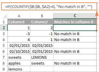
=IF(ISERROR(MATCH($A2, $B$2:$B$10, 0)), "No Match in B", "")

This formula searches for the value in cell A2 within the range B2:B10. If MATCH returns an error (meaning no match is found), ISERROR returns TRUE, and the formula displays “No Match in B”.

4.3 Combining Formulas for Comprehensive Results

To identify both matches and differences, combine the formulas to provide a comprehensive result.

=IF(COUNTIF($B:$B, $A2)=0, "No Match in B", "Match in B")

This formula returns “No Match in B” if the value in A2 is not found in column B, and “Match in B” if it is found.

5. How to Compare Two Lists in Excel and Pull Differences?

When comparing two lists, you might need to extract the values that are different. This involves using functions like VLOOKUP, INDEX-MATCH, or XLOOKUP to locate and retrieve data.

5.1 Leveraging VLOOKUP for Data Extraction

The VLOOKUP function is commonly used to pull matching entries from a lookup table.

=VLOOKUP(D2, $A$2:$B$6, 2, FALSE)

This formula searches for the value in cell D2 within the range A2:A6 and, if a match is found, returns the corresponding value from the second column (B2:B6).

5.2 Using INDEX-MATCH for Enhanced Flexibility

The INDEX-MATCH combination provides more flexibility compared to VLOOKUP.

=INDEX($B$2:$B$6, MATCH($D2, $A$2:$A$6, 0))

Here, MATCH finds the position of the value in cell D2 within the range A2:A6, and INDEX returns the value from the corresponding position in the range B2:B6.

5.3 Employing XLOOKUP for Modern Excel Versions

XLOOKUP is a more modern and versatile function available in Excel 2021 and Excel 365.

=XLOOKUP(D2, $A$2:$A$6, $B$2:$B$6)

This formula searches for the value in cell D2 within the range A2:A6 and returns the corresponding value from the range B2:B6. XLOOKUP is easier to use and offers better error handling compared to VLOOKUP.

6. How to Compare Two Lists and Highlight Differences?

Highlighting matches and differences can help you visualize discrepancies. Conditional formatting is a powerful tool for this task.

6.1 Using Conditional Formatting to Highlight Differences

To highlight cells in column A that have different entries in column B, follow these steps:

1. Select the Range: Select the cells you want to highlight in column A.
2. Open Conditional Formatting: Go to Home > Conditional Formatting > New Rule… > Use a formula to determine which cells to format.
3. Enter the Formula: Enter the following formula:

=$B2<>$A2

1. Set the Format: Click Format to choose the fill color for highlighting the differences.

6.2 Highlighting Unique Entries in Each List

To highlight unique entries in each list, use COUNTIF in conditional formatting rules.

1. Highlight Unique Values in List 1 (Column A):

=COUNTIF($C$2:$C$5, $A2)=0

1. Highlight Unique Values in List 2 (Column C):

=COUNTIF($A$2:$A$6, $C2)=0

Apply these formulas using the same conditional formatting steps as above, but select the appropriate columns.

6.3 Highlighting Matches Between Two Columns

To highlight matches, adjust the COUNTIF formulas to identify entries that exist in both lists.

1. Highlight Matches in List 1 (Column A):

=COUNTIF($C$2:$C$5, $A2)>0

1. Highlight Matches in List 2 (Column C):

=COUNTIF($A$2:$A$6, $C2)>0

7. How to Highlight Row Differences and Matches in Multiple Columns?

When working with multiple columns, you can use conditional formatting and the “Go To Special” feature to highlight differences and matches.

7.1 Highlighting Rows with Identical Values

To highlight rows with identical values in all columns, create a conditional formatting rule based on these formulas:

=AND($A2=$B2, $A2=$C2)

Or:

=COUNTIF($A2:$C2, $A2)=3

7.2 Using “Go To Special” to Highlight Differences

The “Go To Special” feature is a quick way to highlight cells with different values in each row.

1. Select the Range: Select the range of cells you want to compare (e.g., A2:C8).
2. Open “Go To Special”: Go to Home > Find & Select > Go To Special….
3. Select “Row Differences”: Choose Row differences and click OK.
4. Apply Highlighting: The cells with different values will be selected. Apply a fill color to highlight them.

8. How to Compare Two Individual Cells in Excel?

Comparing two individual cells is straightforward using the IF function.

8.1 Using IF for Simple Cell Comparison

To compare cells A1 and C1, use the following formulas:

For matches:

=IF(A1=C1, "Match", "")

For differences:

=IF(A1<>C1, "Difference", "")

9. What Are the Advantages of a Formula-Free Method to Compare Two Columns?

While Excel formulas are powerful, formula-free methods, such as using add-ins like Ablebits Ultimate Suite, offer several advantages:

• Ease of Use: Add-ins provide intuitive interfaces that simplify complex tasks.
• Efficiency: They can handle large datasets more efficiently than complex formulas.
• Comprehensive Features: Add-ins often include additional features like highlighting, status columns, and more.

9.1 Steps to Compare Two Lists Using Ablebits Ultimate Suite

Here’s how to compare two lists using the Compare Two Tables tool in Ablebits Ultimate Suite:

1. Select Compare Tables: Click the Compare Tables button on the Ablebits Data tab.
2. Select Lists: Select the first list and click Next, then select the second list and click Next.
3. Choose Data Type: Choose whether to look for Duplicate values (matches) or Unique values (differences) and click Next.
4. Select Columns: Select the columns for comparison and click Next.
5. Choose Action: Choose how to deal with the found items, such as Highlight with color or Identify in the Status column, and click Finish.

10. FAQ: Comparing Two Excel Columns

Q1: How can I compare two columns in Excel to find differences?
A1: Use the IF function with the <> operator to check for differences in each row. For example, =IF(A2<>B2, "Different", "Same").

Q2: How do I perform a case-sensitive comparison in Excel?
A2: Use the EXACT function within the IF function. For example, =IF(EXACT(A2, B2), "Match", "No Match").

Q3: How can I highlight differences between two columns in Excel?
A3: Use conditional formatting with a formula like =$B2<>$A2 to highlight cells in column A that are different from column B.

Q4: How do I find unique values in two columns using Excel?
A4: Use the COUNTIF function to check if values from one column exist in the other. For example, =IF(COUNTIF($B:$B, $A2)=0, "Unique to A", "").

Q5: Can I compare more than two columns in Excel?
A5: Yes, use the AND function with multiple equality checks or the COUNTIF function to compare multiple columns.

Q6: How do I pull matching data from one column to another based on a comparison?
A6: Use functions like VLOOKUP, INDEX-MATCH, or XLOOKUP to locate and retrieve data from another column.

Q7: What is the best way to highlight rows with identical values in multiple columns?
A7: Use conditional formatting with a formula like =AND($A2=$B2, $A2=$C2) or =COUNTIF($A2:$C2, $A2)=3.

Q8: How can I quickly highlight cells with different values in each row of multiple columns?
A8: Use Excel’s “Go To Special” feature, select “Row differences,” and then apply a fill color to the selected cells.

Q9: What are the benefits of using an Excel add-in for comparing columns?
A9: Add-ins like Ablebits Ultimate Suite offer ease of use, efficiency, and comprehensive features, making complex comparisons simpler and faster.

Q10: How do I compare two individual cells in Excel?
A10: Use the IF function with a simple equality check. For example, =IF(A1=C1, "Match", "") or =IF(A1<>C1, "Difference", "").

Comparing two Excel columns to find differences is a crucial skill for data analysis and validation. By using functions like IF, EXACT, COUNTIF, VLOOKUP, INDEX-MATCH, and XLOOKUP, along with conditional formatting, you can efficiently identify discrepancies and ensure data integrity. For a more user-friendly and feature-rich experience, consider using add-ins like Ablebits Ultimate Suite. At COMPARE.EDU.VN, we strive to provide the most comprehensive and reliable information to help you make informed decisions.

Ready to take your Excel skills to the next level? Visit COMPARE.EDU.VN today to explore more detailed guides, software comparisons, and expert tips for all your data analysis needs. Whether you’re a student, professional, or enthusiast, compare.edu.vn is your go-to resource for making informed comparisons and achieving your goals. Contact us at: Address: 333 Comparison Plaza, Choice City, CA 90210, United States. Whatsapp: +1 (626) 555-9090.

Keywords: Excel comparison, compare Excel columns, find differences in Excel, Excel data analysis, COMPARE.EDU.VN, Excel tutorials, data validation.