How To Compare Two Different Columns In Excel

Comparing two different columns in Excel can be a common task for data analysis, validation, and cleaning. At COMPARE.EDU.VN, we help you understand how to effectively compare data in Excel, offering several methods ranging from simple formulas to conditional formatting. This article aims to guide you through the most efficient techniques for performing column comparisons in Excel, enhancing your data handling capabilities, and improving data integrity.

1. Understanding the Need for Column Comparison in Excel

Excel is a powerful tool for data management, but comparing columns manually can be time-consuming and prone to errors. Automating this process is essential for efficient data analysis and decision-making. Here’s why comparing two columns in Excel is valuable:

• Data Validation: Ensure data accuracy by comparing columns for inconsistencies.
• Data Cleaning: Identify and correct discrepancies in your dataset.
• Duplicate Detection: Find and remove duplicate entries to maintain data integrity.
• Change Tracking: Monitor changes between different versions of a spreadsheet.
• Reporting: Highlight differences or matches to generate insightful reports.

2. Basic Techniques: Comparing Two Columns Using Formulas

One of the simplest ways to compare two columns in Excel is by using formulas. These formulas allow you to perform row-by-row comparisons and return results like “Match” or “Not Match.” Here’s how to do it:

2.1. Using the Equals Operator (=)

The equals operator is the most basic method for comparing two columns. It checks if the values in corresponding rows are identical.

• Formula: =A1=B1
• How it Works: This formula returns TRUE if the values in cells A1 and B1 are the same, and FALSE if they are different.
• Example:

	Column A	Column B	Column C (Formula)
Row 1	Apple	Apple	TRUE
Row 2	Banana	Orange	FALSE
Row 3	Cherry	Cherry	TRUE

• Limitations: This method is case-insensitive and treats “Apple” and “apple” as the same.

2.2. Using the IF Function

The IF function allows you to return custom messages based on whether the values match or not.

• Formula: =IF(A1=B1, "Match", "Not Match")
• How it Works: This formula checks if the values in cells A1 and B1 are the same. If they are, it returns “Match”; otherwise, it returns “Not Match.”
• Example:

	Column A	Column B	Column C (Formula)
Row 1	Apple	Apple	Match
Row 2	Banana	Orange	Not Match
Row 3	Cherry	Cherry	Match

• Customization: You can customize the “Match” and “Not Match” messages to suit your specific needs.

2.3. Using the EXACT Function

The EXACT function provides a case-sensitive comparison of two strings.

• Formula: =EXACT(A1, B1)
• How it Works: This formula returns TRUE only if the values in cells A1 and B1 are exactly the same, including case.
• Example:

	Column A	Column B	Column C (Formula)
Row 1	Apple	Apple	TRUE
Row 2	apple	Apple	FALSE
Row 3	Cherry	Cherry	TRUE

• Case Sensitivity: This function is essential when case differences are significant.

2.4. Combining IF and EXACT Functions

To combine case-sensitive comparison with custom messages, you can use the IF and EXACT functions together.

• Formula: =IF(EXACT(A1, B1), "Match", "Not Match")
• How it Works: This formula checks if the values in cells A1 and B1 are exactly the same, including case. If they are, it returns “Match”; otherwise, it returns “Not Match.”
• Example:

	Column A	Column B	Column C (Formula)
Row 1	Apple	Apple	Match
Row 2	apple	Apple	Not Match
Row 3	Cherry	Cherry	Match

• Advanced Use: This method is highly useful when distinguishing between entries based on case.

3. Conditional Formatting for Visual Comparison

Conditional formatting allows you to highlight differences or matches in two columns visually. This method is useful for quick identification of discrepancies.

3.1. Highlighting Duplicate Values

To highlight values that appear in both columns, follow these steps:

1. Select both columns of data.
2. Go to Home > Conditional Formatting > Highlight Cells Rules > Duplicate Values.
3. Choose the formatting style (e.g., fill with red).
4. Click OK.

• Result: All values that are present in both columns will be highlighted.

3.2. Highlighting Unique Values

To highlight values that appear only in one column, follow these steps:

1. Select both columns of data.
2. Go to Home > Conditional Formatting > Highlight Cells Rules > Duplicate Values.
3. In the dialog box, select Unique from the dropdown menu.
4. Choose the formatting style (e.g., fill with green).
5. Click OK.

• Result: All unique values (values that appear only in one column) will be highlighted.

3.3. Creating Custom Rules

For more complex comparisons, you can create custom conditional formatting rules using formulas.

1. Select the range of cells to format (e.g., Column A).
2. Go to Home > Conditional Formatting > New Rule.
3. Select Use a formula to determine which cells to format.
4. Enter a formula that checks for the condition you want to highlight. For example, to highlight values in Column A that are not in Column B, use the formula: =ISNA(MATCH(A1, $B:$B, 0))
5. Click Format and choose the formatting style.
6. Click OK twice.

• Explanation of the Formula:
  • MATCH(A1, $B:$B, 0): This searches for the value in cell A1 within Column B. It returns the row number where the value is found, or #N/A if not found.
  • ISNA(...): This checks if the result of the MATCH function is #N/A. It returns TRUE if the value is not found in Column B, and FALSE if it is found.
  • The conditional formatting will apply the chosen format to cells in Column A where the formula returns TRUE.

4. Advanced Techniques: Using Lookup Functions

Lookup functions like VLOOKUP, HLOOKUP, and XLOOKUP can be used to compare two columns in Excel by searching for values in one column within another.

4.1. Using VLOOKUP to Find Matches

VLOOKUP searches for a value in the first column of a range and returns a value from a specified column in the same row.

• Formula: =IF(ISNA(VLOOKUP(A1, $B:$B, 1, FALSE)), "Not Found", "Found")
• How it Works:
  • VLOOKUP(A1, $B:$B, 1, FALSE): This searches for the value in cell A1 within Column B. If found, it returns the value itself. If not found, it returns #N/A.
  • ISNA(...): This checks if the result of the VLOOKUP function is #N/A. It returns TRUE if the value is not found in Column B, and FALSE if it is found.
  • IF(ISNA(...), "Not Found", "Found"): This returns “Not Found” if the value is not in Column B, and “Found” if it is.
• Example:

	Column A	Column B	Column C (Formula)
Row 1	Apple	Apple	Found
Row 2	Banana	Orange	Not Found
Row 3	Cherry	Cherry	Found

• Absolute Reference: The $B:$B in the formula is an absolute reference, ensuring that the lookup range does not change when you drag the formula down.

4.2. Using XLOOKUP (Modern Alternative)

XLOOKUP is a more versatile and modern lookup function that can perform similar tasks to VLOOKUP but with improved syntax and capabilities.

• Formula: =IF(ISNA(XLOOKUP(A1, $B:$B, $B:$B, "", 0)), "Not Found", "Found")
• How it Works:
  • XLOOKUP(A1, $B:$B, $B:$B, "", 0): This searches for the value in cell A1 within Column B. If found, it returns the value from Column B. If not found, it returns an empty string (“”).
  • ISNA(...): This checks if the result of the XLOOKUP function is an error (i.e., the value was not found).
  • IF(ISNA(...), "Not Found", "Found"): This returns “Not Found” if the value is not in Column B, and “Found” if it is.
• Benefits of XLOOKUP:
  • More flexible syntax.
  • Can return values from any column, not just to the right of the lookup column.
  • Handles errors more gracefully.

5. Comparing Multiple Columns

Sometimes, you may need to compare more than two columns. Excel provides methods to compare multiple columns using a combination of formulas and functions.

5.1. Using IF and AND Functions

To check if values in multiple columns are identical, you can use the IF and AND functions.

• Formula: =IF(AND(A1=B1, A1=C1), "Match", "Not Match")
• How it Works: This formula checks if the values in cells A1, B1, and C1 are all the same. If they are, it returns “Match”; otherwise, it returns “Not Match.”
• Example:

	Column A	Column B	Column C	Column D (Formula)
Row 1	Apple	Apple	Apple	Match
Row 2	Banana	Orange	Banana	Not Match
Row 3	Cherry	Cherry	Cherry	Match

• Scalability: You can extend this formula to include more columns by adding more conditions to the AND function.

5.2. Using COUNTIF for Multiple Columns

The COUNTIF function can be used to count how many times a value appears in a range of cells.

• Formula: =IF(COUNTIF($A$1:$C$1, A1)=3, "Match", "Not Match")
• How it Works:
  • COUNTIF($A$1:$C$1, A1): This counts how many times the value in cell A1 appears within the range A1 to C1.
  • IF(COUNTIF(...)=3, "Match", "Not Match"): If the count is equal to 3 (the number of columns being compared), it returns “Match”; otherwise, it returns “Not Match.”
• Flexibility: This method is useful when comparing a value against multiple columns and determining if it is present in all of them.

6. Practical Examples and Use Cases

To illustrate the practical applications of these techniques, let’s consider a few use cases:

6.1. Comparing Product Lists

Imagine you have two lists of products in different spreadsheets and want to identify which products are present in both lists.

• Scenario:
  • Sheet1: Product List A
  • Sheet2: Product List B
• Method: Use the VLOOKUP or XLOOKUP function in Sheet1 to check if each product is present in Sheet2.
• Formula (in Sheet1): =IF(ISNA(XLOOKUP(A1, 'Sheet2'!$A:$A, 'Sheet2'!$A:$A, "", 0)), "Not Found", "Found")
• Benefit: Quickly identify which products are common between the two lists.

6.2. Validating Data Entries

You have a database of customer information and want to ensure that the email addresses in two columns (e.g., “Email” and “Backup Email”) are consistent.

• Scenario:
  • Column A: Email
  • Column B: Backup Email
• Method: Use the IF and EXACT functions to compare the email addresses.
• Formula: =IF(EXACT(A1, B1), "Match", "Not Match")
• Benefit: Ensure data accuracy by identifying discrepancies in email addresses.

6.3. Tracking Changes in Inventory

You have two versions of an inventory list and want to track the changes in stock levels.

• Scenario:
  • Sheet1: Inventory List (Original)
  • Sheet2: Inventory List (Updated)
• Method: Use a combination of VLOOKUP and IF functions to compare the stock levels.
• Formulas:
  • In Sheet2, use VLOOKUP to retrieve the original stock level from Sheet1: =VLOOKUP(A1, 'Sheet1'!$A:$B, 2, FALSE) (assuming product names are in Column A and stock levels in Column B).
  • Compare the current stock level with the original stock level: =IF(B1='Sheet1'!B1, "No Change", "Changed")
• Benefit: Easily track changes in inventory levels between the two versions of the list.

7. Tips and Best Practices

When comparing two columns in Excel, keep the following tips and best practices in mind:

• Consistency: Ensure that the data types in both columns are consistent. Comparing text with numbers may lead to incorrect results.
• Clean Data: Remove any leading or trailing spaces from your data using the TRIM function. This can help avoid false negatives in your comparisons.
• Case Sensitivity: Be aware of whether your comparison needs to be case-sensitive. Use the EXACT function when case matters.
• Error Handling: Use the ISNA function to handle errors that may arise from lookup functions like VLOOKUP and XLOOKUP.
• Absolute References: Use absolute references ($) in your formulas to prevent the lookup ranges from changing when you drag the formulas down.
• Test Your Formulas: Always test your formulas on a small sample of data to ensure they are working correctly before applying them to the entire dataset.
• Use Helper Columns: For complex comparisons, consider using helper columns to break down the problem into smaller, more manageable steps.

8. Common Mistakes to Avoid

• Ignoring Case Sensitivity: Forgetting to use the EXACT function when case matters can lead to incorrect results.
• Not Using Absolute References: Failing to use absolute references in lookup formulas can cause the lookup ranges to change unexpectedly.
• Comparing Different Data Types: Comparing text with numbers or dates can lead to incorrect results. Ensure that the data types are consistent.
• Overlooking Leading/Trailing Spaces: Leading or trailing spaces can cause comparisons to fail. Use the TRIM function to remove these spaces.
• Not Handling Errors: Not handling errors that may arise from lookup functions can lead to incorrect results or broken formulas.

9. Automating Column Comparisons with VBA

For advanced users, VBA (Visual Basic for Applications) can be used to automate the process of comparing two columns in Excel. Here’s a basic example of how to compare two columns and highlight the differences:

Sub CompareColumns()
    Dim ws As Worksheet
    Dim LastRow As Long
    Dim i As Long

    ' Set the worksheet
    Set ws = ThisWorkbook.Sheets("Sheet1") ' Change "Sheet1" to your sheet name

    ' Get the last row with data in Column A
    LastRow = ws.Cells(ws.Rows.Count, "A").End(xlUp).Row

    ' Loop through the rows
    For i = 1 To LastRow
        ' Compare the values in Column A and Column B
        If ws.Cells(i, "A").Value <> ws.Cells(i, "B").Value Then
            ' Highlight the cells if they are different
            ws.Cells(i, "A").Interior.Color = vbYellow
            ws.Cells(i, "B").Interior.Color = vbYellow
        End If
    Next i

    MsgBox "Comparison complete!"
End Sub

• How it Works:
  • This VBA code loops through the rows of the specified worksheet and compares the values in Column A and Column B.
  • If the values are different, it highlights both cells in yellow.
• Customization:
  • Change "Sheet1" to the name of your worksheet.
  • Modify the If condition to perform more complex comparisons.
  • Adjust the highlighting color or other formatting options as needed.

10. Utilizing Third-Party Add-Ins

Several third-party add-ins can enhance your ability to compare columns in Excel. These add-ins often provide additional features and functionalities that are not available in the native Excel application. Here are a few popular options:

• Ablebits Ultimate Suite for Excel: This suite includes a “Compare Two Sheets” tool that can quickly identify differences between two worksheets or columns.
• ASAP Utilities: This add-in offers a variety of tools, including a “Compare columns” feature that can highlight differences, find duplicates, and more.
• Spreadsheet Compare: This Microsoft tool is designed to compare two Excel files and highlight the differences in data, formulas, and formatting.

These add-ins can save you time and effort by automating complex comparison tasks and providing advanced features for data analysis.

11. Addressing Common Scenarios

11.1. Comparing Columns with Different Lengths

When the columns you are comparing have different lengths, you need to adjust your formulas to handle the potential errors that may arise. One way to do this is to use the IFERROR function.

• Scenario: Column A has more rows than Column B.
• Formula: =IFERROR(IF(A1=B1, "Match", "Not Match"), "Not in Column B")
• How it Works: This formula first attempts to compare the values in cells A1 and B1. If an error occurs (e.g., because there is no corresponding value in Column B), the IFERROR function returns “Not in Column B.”

11.2. Comparing Columns with Blanks

When comparing columns that contain blank cells, you may want to treat blank cells as either matching or not matching each other.

• Scenario: You want to treat blank cells as matching each other.
• Formula: =IF(OR(AND(ISBLANK(A1), ISBLANK(B1)), A1=B1), "Match", "Not Match")
• How it Works: This formula checks if both cells A1 and B1 are blank or if their values are equal. If either condition is true, it returns “Match”; otherwise, it returns “Not Match.”

11.3. Comparing Columns with Numbers Formatted as Text

Sometimes, numbers in Excel may be formatted as text, which can cause comparisons to fail. To address this issue, you can use the VALUE function to convert the text to numbers before comparing them.

• Scenario: Numbers in Column A are formatted as text.
• Formula: =IF(VALUE(A1)=B1, "Match", "Not Match")
• How it Works: This formula converts the value in cell A1 to a number using the VALUE function before comparing it with the value in cell B1.

12. Integrating Column Comparisons with Other Excel Functions

Column comparisons can be integrated with other Excel functions to perform more complex data analysis tasks. Here are a few examples:

12.1. Using with Data Validation

You can use column comparisons in conjunction with data validation to ensure that users enter valid data into a spreadsheet.

• Scenario: You want to ensure that the values entered in Column C match the values in Column A.
• Method:
  1. Select Column C.
  2. Go to Data > Data Validation.
  3. In the Settings tab, select Custom from the Allow dropdown menu.
  4. Enter the formula =A1=C1 in the Formula field.
  5. In the Error Alert tab, customize the error message that will be displayed when a user enters an invalid value.

12.2. Using with Pivot Tables

Column comparisons can be used to create calculated fields in pivot tables that show the differences or matches between two columns.

• Scenario: You want to create a pivot table that shows the differences between the values in Column A and Column B.
• Method:
  1. Create a pivot table based on your data.
  2. In the pivot table, add the columns to the Rows or Columns area.
  3. Create a calculated field using the formula =ColumnA-ColumnB.
  4. Format the calculated field to show the differences between the two columns.

13. Best Practices for Large Datasets

When working with large datasets, it’s important to optimize your formulas and techniques to ensure that Excel performs efficiently. Here are a few best practices:

• Use Array Formulas Sparingly: Array formulas can be powerful, but they can also slow down Excel, especially with large datasets. Use them sparingly and consider alternative methods when possible.
• Avoid Volatile Functions: Volatile functions like NOW() and RAND() recalculate every time the worksheet is changed, which can slow down Excel. Avoid using these functions in your comparison formulas if possible.
• Use Excel Tables: Excel tables can improve performance by automatically adjusting the ranges in your formulas when you add or remove data.
• Consider Power Query: Power Query is a powerful tool for importing, transforming, and comparing data from multiple sources. It can handle large datasets more efficiently than traditional Excel formulas.

14. Frequently Asked Questions (FAQ)

Q1: How do I compare two columns in Excel for exact matches?

A: Use the =IF(EXACT(A1, B1), "Match", "Not Match") formula to perform a case-sensitive comparison.

Q2: How can I highlight differences between two columns?

A: Use conditional formatting with a formula like =A1<>B1 to highlight cells that do not match.

Q3: How do I compare two columns and return a value from a third column?

A: Use the XLOOKUP function: =XLOOKUP(A1, $B:$B, $C:$C, "Not Found") to search for values in Column A within Column B and return corresponding values from Column C.

Q4: Can I compare two columns if they have different lengths?

A: Yes, use IFERROR with your comparison formula to handle cases where a value is missing in one of the columns.

Q5: How do I compare multiple columns to find identical values?

A: Use the AND function with multiple equality checks: =IF(AND(A1=B1, A1=C1, A1=D1), "Match", "Not Match").

Q6: What is the best way to compare two large datasets in Excel?

A: Consider using Power Query or third-party add-ins designed for efficient data comparison.

Q7: How do I compare columns with numbers formatted as text?

A: Use the VALUE function to convert text to numbers: =IF(VALUE(A1)=VALUE(B1), "Match", "Not Match").

Q8: Can I automate column comparisons in Excel?

A: Yes, use VBA to write a macro that loops through the rows and performs the comparisons.

Q9: How do I handle blank cells when comparing columns?

A: Use the ISBLANK function to check for blank cells and adjust your formulas accordingly.

Q10: What are some common mistakes to avoid when comparing columns in Excel?

A: Avoid ignoring case sensitivity, not using absolute references, comparing different data types, and overlooking leading/trailing spaces.

Conclusion

Comparing two different columns in Excel is a fundamental task for data analysis and management. By mastering the techniques outlined in this article, you can efficiently identify differences, validate data, and ensure data integrity. Whether you’re using simple formulas, conditional formatting, lookup functions, or VBA, COMPARE.EDU.VN has provided you with the knowledge to tackle any column comparison challenge.

Ready to take your Excel skills to the next level? Visit COMPARE.EDU.VN at 333 Comparison Plaza, Choice City, CA 90210, United States, or contact us via WhatsApp at +1 (626) 555-9090. Explore our comprehensive resources and discover how we can help you make informed decisions based on accurate data comparisons. Don’t just compare – compare.edu.vn!

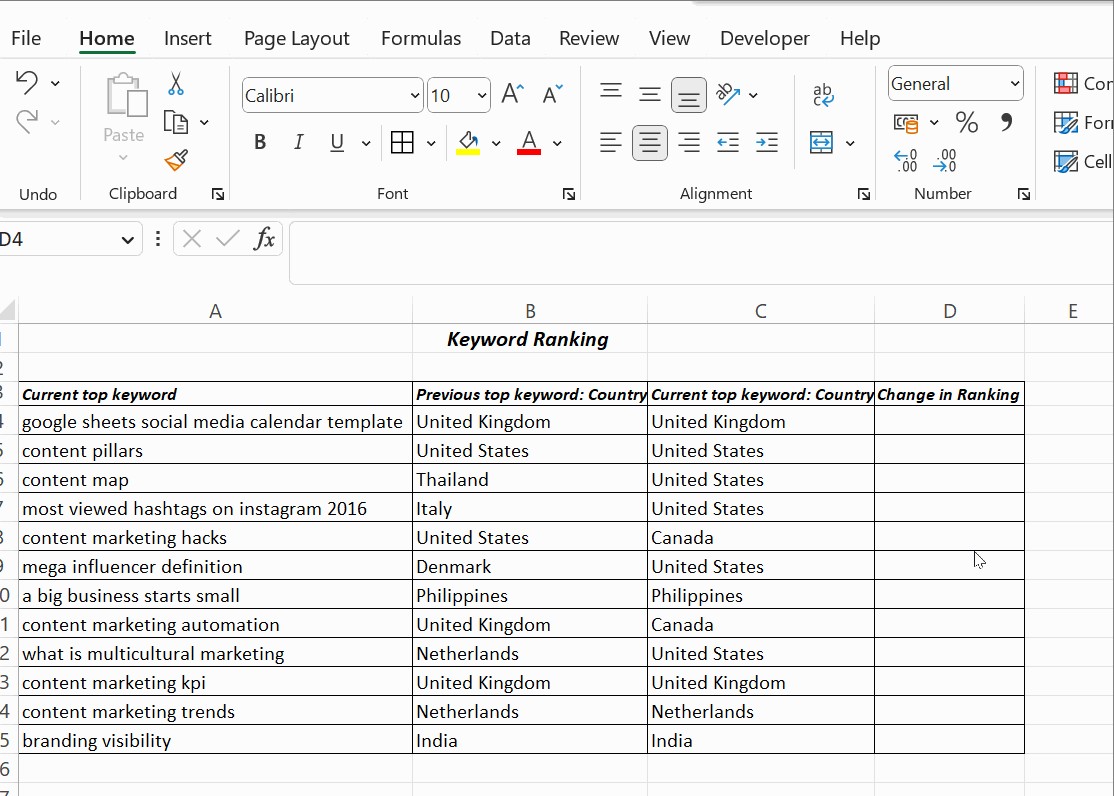Excel Column Comparison Using Formulas