How Do You Compare Two Curves? A Comprehensive Guide

Comparing two curves involves assessing the similarities and differences in their shapes, magnitudes, and trends. This guide from COMPARE.EDU.VN provides a detailed, SEO-optimized approach, utilizing statistical methods and practical examples, to empower you to effectively compare curves. By understanding the key concepts and techniques outlined here, you’ll gain the ability to make informed decisions based on comprehensive curve analysis.

1. What is Curve Comparison and Why is it Important?

Curve comparison is the process of analyzing two or more graphical representations of data to identify similarities, differences, and trends. This comparison is crucial in various fields, from scientific research and engineering to finance and data analysis. It allows for data validation, trend identification, and performance evaluation.

In scientific research, comparing curves can help researchers determine the effectiveness of different treatments or the impact of various conditions on a system. For instance, in a clinical trial, researchers might compare the survival curves of patients receiving a new drug versus those receiving a placebo. This helps them assess whether the new drug significantly improves patient survival rates. According to a study by the National Institutes of Health (NIH) in 2023, curve comparison is fundamental in evaluating treatment outcomes and understanding disease progression.

In engineering, curve comparison is used to evaluate the performance of different designs or materials. For example, engineers might compare the stress-strain curves of different materials to determine which is best suited for a particular application. According to research from the American Society of Mechanical Engineers (ASME) in 2024, precise curve comparison aids in material selection and structural integrity assessment.

In finance, comparing curves is essential for analyzing market trends and investment performance. For instance, analysts might compare the stock price curves of two companies to identify potential investment opportunities. Data from the Securities and Exchange Commission (SEC) indicates that comparing historical trends can provide crucial insights into future performance.

2. What are Common Methods for Comparing Curves?

Several methods exist for comparing curves, each with its strengths and weaknesses. The choice of method depends on the nature of the data, the specific research question, and the desired level of detail. These methods can be broadly classified into visual inspection, statistical tests, and mathematical modeling.

Visual Inspection: The simplest method involves visually comparing the curves. While this can provide a quick overview, it is subjective and lacks statistical rigor. It’s best used as a preliminary step to identify potential areas of interest before applying more quantitative methods. Visual inspection can be misleading due to human perception biases, emphasizing the need for analytical tools.
Statistical Tests: Statistical tests provide a more objective way to compare curves. Common tests include:
- Chi-squared Test: A versatile statistical test used to determine if there is a significant association between two categorical variables. In the context of curve comparison, it can be adapted to compare the overall fit of two curves by assessing the sum of squared differences between them, relative to the expected differences based on random sampling. This method requires a correction for small sample sizes, typically found in biomedical research, to account for deviations from normality.
- T-Test: A statistical test used to determine if there is a significant difference between the means of two groups. It is often used to compare individual data points on two curves at specific X-values, assessing whether the means are statistically different. A Welch’s corrected t-test is particularly useful as it does not assume equal standard deviations between the two sets of data.
- ANOVA (Analysis of Variance): Used to compare the means of two or more groups. However, it is not ideal for comparing arbitrary curves as it requires assumptions about how the curve values change.
- Kolmogorov-Smirnov Test: A non-parametric test used to determine if two samples come from the same distribution. It’s useful for comparing curves without making assumptions about the underlying distribution.
- Area Under the Curve (AUC): A measure of the overall performance of a curve. Comparing AUC values can indicate which curve performs better overall.
- Root Mean Square Error (RMSE): A statistical measure of the magnitude of the difference between values predicted by a model and the values actually observed. It’s used to quantify the accuracy of a curve fit.
Mathematical Modeling: This involves fitting mathematical models to the curves and comparing the model parameters. This method is useful when the curves can be described by well-defined mathematical functions. Comparing parameters can provide insights into the underlying processes that generate the curves. For example, in pharmacokinetics, comparing the elimination rates of a drug under different conditions can help understand how the drug is metabolized.

3. How to Use the Chi-Squared Method for Curve Comparison

The Chi-squared method is a versatile tool for comparing curves. Here’s a detailed guide on how to use it, with a focus on the modified Chi-squared method:

3.1. Understanding the Basics

The Chi-squared test is used to determine whether the observed differences between two curves are statistically significant or due to random chance. It is particularly useful when comparing experimental data against expected values.

Formula: The basic Chi-squared formula is:

χ2=∑(Oi−Ei)2σi2

Where:
- Oi is the observed value at point i.
- Ei is the expected value at point i.
- σi is the standard deviation of the observed value at point i.
Degrees of Freedom: The degrees of freedom (df) is the number of independent pieces of information used to calculate the statistic. For curve comparison, df is often the number of points being compared (M).
P-value: The p-value is the probability of observing a test statistic as extreme as, or more extreme than, the statistic obtained from the sample, assuming the null hypothesis is true. A small p-value (typically less than 0.05) indicates that the differences between the curves are statistically significant.

3.2. Scenarios for Curve Comparison

There are two primary scenarios when using the Chi-squared method for curve comparison:

Scenario 1: One Measurement at Each X with Known Standard Deviation
In this scenario, you have a single measurement at each point and a known standard deviation (σi) for each measurement. The Chi-squared formula becomes:

χi2=(Oia−Oib)2σidiff2

Where:
- Oia is the observed value for curve a at point i.
- Oib is the observed value for curve b at point i.
- σidiff is the standard deviation of the difference, calculated as:
σidiff=σia2+σib2
Scenario 2: N Measurements at Each X, Giving Mean and Standard Error
In this scenario, you have N independent measurements at each point, allowing you to calculate a mean (Oi) and standard error (SEi) for each point. The Chi-squared formula becomes:

χi2=(Oia−Oib)2SEidiff2

Where:
- Oia is the mean value for curve a at point i.
- Oib is the mean value for curve b at point i.
- SEidiff is the standard error of the difference, calculated as:
SEidiff=SEia2+SEib2

And SEij is the standard error of each measurement, calculated from the measured standard deviation (σij):

SEij=σijNij

3.3. Correcting for Small Sample Sizes

When dealing with small sample sizes (N ≤ 20), the assumption of normality may not hold. To correct for this, use the t-distribution to calculate a corrected Chi-squared value for each pair of points.

Calculate t-value:

ti=Oia−OibSEidiff
Determine Degrees of Freedom (dFt):
- If the number of measurements is the same for both curves (N), dFt = 2N – 2.
- If the number of measurements is different, dFt = 2Nsmaller – 2, where Nsmaller is the smaller of the two N values.
Calculate Probability (pi) using t-distribution:
Use a t-distribution calculator or function in a spreadsheet program to find the probability associated with the calculated t-value and degrees of freedom.
Calculate Corrected Chi-Squared Value:
Use an inverse Chi-squared calculator or function with df = 1 to find the corrected Chi-squared value:

p i and dF = 1 → χ2−distribution χ corr,i2

3.4. Calculating Overall Statistical Significance

To calculate the overall p-value for the difference between the two curves, sum the corrected Chi-squared values:

χsum2=∑i=1Mχcorr,i2

Then, use a Chi-squared calculator with df = M to find the overall p-value.

χsum2 and dFcurves (M) → χ2−distribution p overall

3.5. Using Excel for Chi-Squared Calculations

Microsoft Excel can be used to perform these calculations. Here’s a step-by-step guide:

Scenario 1: N = 1 with SD
- Column A: Enter Xi, the X-values for the two curves.
- Column B: Enter Oia, the measured value of Y for curve a.
- Column C: Enter SDia, the standard deviation of point i for curve a.
- Column D: Enter Oib, the measured value of Y for curve b.
- Column E: Enter SDib, the standard deviation of point i for curve b.
- Column G: Calculate the absolute difference between the means: = ABS(Di-Bi)
- Column H: Calculate the standard deviation of the difference: = SQRT(Ci^2+Ei^2)
- Column I: Calculate the individual Chi-squared values: = (Gi/Hi)^2
Scenario 2: N > 1 with Mean and SE
- Column A: Enter Xi, the X-values for the two curves.
- Column B: Enter Oia, the mean of Y for curve a.
- Column C: Enter SDia, the standard deviation of point i for curve a.
- Column D: Enter Nia, the number of measurements for point i for curve a.
- Column E: Enter SEia, the standard error of point i for curve a.
- Column F: Enter Oib, the mean of Y for curve b.
- Column G: Enter SDib, the standard deviation of point i for curve b.
- Column H: Enter Nib, the number of measurements for point i for curve b.
- Column I: Enter SEib, the standard error of point i for curve b.
- Column K: Calculate the absolute difference between the means: = ABS(Fi-Bi)
- Column L: Calculate the standard error of the difference: = SQRT(Ei^2+Ii^2)
- Column M: Calculate the t-value: = Ki/Li
- Column N: Determine N for dF calculation: = IF(HiO: Calculate dF for t-calculation: = 2*Ni-2`
- Column P: Calculate the probability from t and dF: = T.DIST.2T(Mi,Oi)
- Column Q: Calculate the corrected χi2: = CHISQ.INV.RT(Pi,1)
Calculating the Overall P-Value in Excel
- For N = 1 with SD, use Col L for χi2 and Col I for χcorr,i2.
- For N > 1 with mean and SE, use Col T for χi2 and Col Q for χcorr,i2.
- Cell X2: Calculate the sum of χi2: = SUM(Y3:Ym), where m is the row containing the last pair of points.
- Cell X3: Determine df for χi2: = COUNT(Y3:Ym)
- Cell X4: Calculate the overall p-value: = 1-CHISQ.DIST(X2,X3,TRUE)

3.6. Example Data Analysis

Consider the example of comparing the relative activation of wild-type FGFR3 and the G380R mutant. Suppose you have the following data:

Ligand (nM)	Wild Type FGFR3 (Mean)	Wild Type FGFR3 (SE)	G380R Mutant FGFR3 (Mean)	G380R Mutant FGFR3 (SE)
0	0.515	0.122	1.166	0.227
5	0.309	0.089	0.822	0.172
25	0.149	0.064	0.708	0.153
50	0.205	0.073	0.673	0.148
125	0.151	0.064	0.390	0.102
500	0.195	0.071	0.331	0.093
1250	0.338	0.094	0.241	0.079
2500	0.415	0.106	0.395	0.103

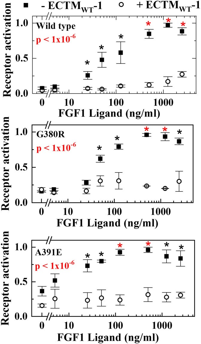
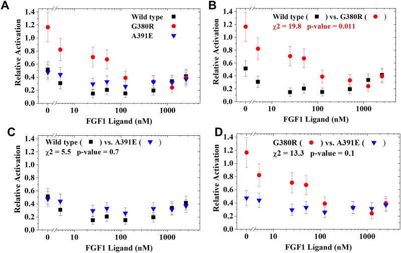
Using the steps outlined above, you can calculate the Chi-squared values, t-values, degrees of freedom, and the overall p-value to determine if the differences between the curves are statistically significant.

4. What are the Advantages and Limitations of the Chi-Squared Method?

4.1. Advantages

Versatility: Applicable to various types of data and experimental designs.
Ease of Implementation: Can be easily implemented using spreadsheet programs like Excel.
Correction for Small Sample Sizes: The modified Chi-squared method corrects for deviations from normality when dealing with small sample sizes.
Objective Statistical Significance: Provides an objective measure of statistical significance, reducing subjective interpretation.

4.2. Limitations

Data Requirements: Requires data at the same X-values for both curves.
Normality Assumption: Assumes that data approaches a Gaussian distribution for large N.
Non-Zero Standard Deviations: SD/SE values cannot be zero for both curves.
Pairwise Comparisons: Limited to pairwise comparisons; corrections must be made for multiple comparisons.

5. What is Post Hoc Analysis and How to Perform It?

Post hoc analysis involves examining specific data points that contribute most to the overall difference between the curves. The p-values calculated at each X-value can be used to determine which points are significantly different.

5.1. Bonferroni Correction

To correct for multiple comparisons, use the Bonferroni correction:

αcorr=αoverall/M

Where αoverall is the desired total Type 1 error rate (typically 0.05) and M is the number of pairs of points being compared.

A statistically significant difference between curves can be identified even when none of the differences between the individual points reach the level of significance after the Bonferroni correction.

5.2. Benjamini-Hochberg Procedure

For curves with many comparisons, the Benjamini-Hochberg procedure can be more appropriate. This method controls the false discovery rate (FDR), which is the expected proportion of false positives among the rejected hypotheses.

Rank the P-values: Sort the p-values obtained from the individual comparisons in ascending order.
Calculate Critical Values: For each p-value, calculate a critical value using the formula:

Critical Valuei=i/m∗α

Where:
- i is the rank of the p-value
- m is the total number of comparisons
- α is the desired FDR level (e.g., 0.05)
Compare and Determine Significance: Compare each p-value to its corresponding critical value. Find the largest p-value that is less than or equal to its critical value. All p-values less than or equal to this p-value are considered significant.

The Benjamini-Hochberg procedure provides a less stringent correction for multiple comparisons compared to the Bonferroni correction, making it suitable for exploratory analyses where controlling the FDR is more important than minimizing the risk of Type I errors.

6. Real-World Applications of Curve Comparison

Curve comparison is used across numerous disciplines to inform decisions and gain insights from data.

Medicine and Healthcare: Analyzing survival curves, dose-response curves, and patient recovery rates to evaluate treatment effectiveness and drug efficacy.
Engineering and Manufacturing: Comparing stress-strain curves of different materials, performance curves of different designs, and failure rates to optimize designs and select the best materials.
Finance and Economics: Analyzing stock price trends, market growth curves, and economic indicators to identify investment opportunities and predict market trends.
Environmental Science: Comparing pollution levels over time, species distribution curves, and climate change impacts to assess environmental health and develop effective conservation strategies.

7. Practical Tips for Effective Curve Comparison

To ensure accurate and meaningful curve comparisons, consider these practical tips:

Ensure Data Quality: Verify the accuracy and reliability of the data used to generate the curves.
Use Appropriate Methods: Select the comparison method that best fits the data type and research question.
Consider Sample Size: Account for the impact of sample size on the statistical significance of the results.
Correct for Multiple Comparisons: Apply appropriate corrections to maintain the desired level of statistical significance.
Document Thoroughly: Document all steps of the comparison process, including data sources, methods, and assumptions.

8. Advanced Techniques for Curve Comparison

For more complex curve comparison scenarios, consider these advanced techniques:

Dynamic Time Warping (DTW): A technique used to align time series data that may have variations in speed or timing.
Functional Data Analysis (FDA): A statistical framework for analyzing data that are functions of time or space, allowing for more sophisticated comparisons of curve shapes and features.
Machine Learning Methods: Employ machine learning algorithms to identify patterns and differences between curves, such as clustering algorithms to group similar curves and classification algorithms to predict curve membership.

9. Future Trends in Curve Comparison

The field of curve comparison continues to evolve with advancements in technology and data analysis techniques.

AI and Machine Learning: Integration of artificial intelligence (AI) and machine learning algorithms to automate curve comparison and identify complex patterns.
Big Data Analytics: Analysis of large datasets to compare curves across diverse populations and conditions.
Interactive Visualization: Development of interactive tools for visualizing and comparing curves in real-time, facilitating collaborative analysis and decision-making.
Cloud-Based Solutions: Cloud-based platforms for storing, processing, and analyzing curve data, enabling global collaboration and access to advanced analytical tools.

10. FAQs About Curve Comparison

1. What does curve fitting achieve in curve comparison?

Curve fitting helps simplify complex curves by approximating them with mathematical functions. This allows for easier comparison of curve parameters and identification of underlying trends.

2. How do I determine the best method for comparing two curves?

The best method depends on the nature of the data, the research question, and the desired level of detail. Consider factors such as sample size, data distribution, and the presence of noise.

3. What is the significance of a small p-value in curve comparison?

A small p-value (typically less than 0.05) indicates that the differences between the curves are statistically significant and not due to random chance.

4. How can I correct for multiple comparisons when comparing multiple curves?

Use methods such as the Bonferroni correction or the Benjamini-Hochberg procedure to adjust the significance level and control the risk of Type I errors.

5. What are some common pitfalls to avoid when comparing curves?

Avoid subjective interpretations, ensure data quality, use appropriate methods, and account for sample size and multiple comparisons.

6. How do I handle curves with different lengths or sampling intervals?

Use techniques such as interpolation or dynamic time warping (DTW) to align the curves before comparison.

7. What role does visualization play in curve comparison?

Visualization helps identify patterns, trends, and differences between curves. Use appropriate plots and charts to effectively communicate the results of the comparison.

8. How can I use curve comparison in predictive modeling?

Curve comparison can be used to identify features and patterns that can be used to build predictive models. Use techniques such as regression analysis and machine learning to develop models that accurately predict future trends.

9. What are some open-source tools available for curve comparison?

Tools such as R, Python, and MATLAB offer a wide range of functions and libraries for curve comparison.

10. How can I stay updated on the latest advancements in curve comparison techniques?

Follow relevant publications, attend conferences, and engage with online communities and forums to stay informed about the latest developments in the field.

Curve comparison is a powerful tool for extracting meaningful insights from data. By understanding the various methods, techniques, and considerations, you can effectively compare curves and make informed decisions.

Conclusion

The ability to compare two curves effectively is essential for informed decision-making across diverse fields. This comprehensive guide from COMPARE.EDU.VN has equipped you with the knowledge and tools to analyze curves using visual inspection, statistical tests, and mathematical modeling.

Ready to take your curve comparison skills to the next level? Visit COMPARE.EDU.VN today for more in-depth analyses, comparisons, and resources. Whether you’re a student, researcher, engineer, or data analyst, COMPARE.EDU.VN provides the tools and insights you need to succeed.

Contact Us:

Address: 333 Comparison Plaza, Choice City, CA 90210, United States

WhatsApp: +1 (626) 555-9090

Website: compare.edu.vn

Fig 1. Simulated pairs of curves with standard errors illustrating that any pair of arbitrary curves can be compared to produce a p-value using the described method.