How to Compare Two Columns With Different Values in Excel

Comparing two columns with different values in Excel can be a time-consuming task, especially with large datasets. At COMPARE.EDU.VN, we provide detailed guides and tools to simplify this process, offering solutions for identifying matches, differences, and unique entries. Discover various Excel techniques to efficiently analyze your data. Learn about data comparison, cell comparison, and list comparison.

1. Understanding the Basics of Column Comparison in Excel

Comparing columns in Excel involves identifying similarities and differences between data sets. This is a fundamental skill for data analysis, reporting, and decision-making. Whether you need to find matching entries, unique values, or inconsistencies, Excel offers several powerful methods to achieve your goals.

1.1 Why Compare Columns in Excel?

Column comparison is crucial for several reasons:

Data Validation: Ensure data accuracy by verifying that information in different columns matches.
Identifying Discrepancies: Spot errors or inconsistencies in your data.
Merging Data: Combine data from different sources by identifying common entries.
Reporting and Analysis: Extract meaningful insights from your data by comparing different categories or metrics.
Decision Making: Making informed decisions based on accurate and compared data.

1.2 Common Scenarios for Column Comparison

Here are some typical scenarios where column comparison is essential:

Inventory Management: Comparing stock levels in different warehouses to identify shortages or surpluses.
Sales Analysis: Comparing sales data across different regions or time periods to identify trends.
Customer Relationship Management (CRM): Comparing customer data from different sources to identify duplicates or inconsistencies.
Financial Analysis: Comparing financial statements from different periods to identify changes in performance.
Academic Research: Comparing research data and finding the correlations.

1.3 Key Considerations Before You Start

Before diving into column comparison, keep these points in mind:

Data Type: Ensure that the data types in the columns you’re comparing are consistent (e.g., numbers, text, dates).
Case Sensitivity: Decide whether your comparison should be case-sensitive (e.g., “Apple” vs. “apple”).
Whitespace: Be aware of leading or trailing spaces in your data, as these can affect comparison results.
Error Handling: Plan for potential errors or inconsistencies in your data and how you’ll handle them.

2. Methods for Comparing Two Columns in Excel

Excel offers several techniques for comparing columns, each with its own strengths and weaknesses. Here are some of the most effective methods:

2.1 Conditional Formatting

Conditional formatting allows you to visually highlight differences or matches between columns.

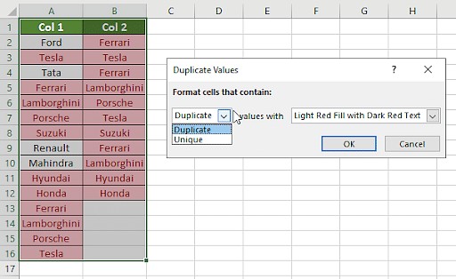
2.1.1 Highlighting Duplicate Values

Select the columns you want to compare.
Go to Home > Conditional Formatting > Highlight Cells Rules > Duplicate Values.
Choose a formatting style (e.g., fill color) for duplicate values.
Click OK.

This method highlights all matching entries in both columns, making it easy to spot duplicates.

Alt Text: Highlighting duplicate values in excel using conditional formatting.

2.1.2 Highlighting Unique Values

Select the columns you want to compare.
Go to Home > Conditional Formatting > Highlight Cells Rules > Duplicate Values.
In the dialog box, choose “Unique” from the dropdown menu.
Choose a formatting style for unique values.
Click OK.

This method highlights entries that appear only in one of the selected columns.

Alt Text: Highlighting unique values in excel using conditional formatting.

2.1.3 Creating Custom Rules

You can create custom conditional formatting rules to highlight cells based on more complex criteria.

Select the columns you want to compare.
Go to Home > Conditional Formatting > New Rule.
Choose “Use a formula to determine which cells to format”.
Enter a formula that compares the corresponding cells in the two columns (e.g., =A1<>B1).
Choose a formatting style.
Click OK.

This allows you to highlight cells where the values are different, regardless of whether they are duplicates or unique.

2.2 Using the Equals Operator (=)

The equals operator provides a simple way to compare individual cells in two columns.

2.2.1 Basic Comparison

In a new column, enter the formula =A1=B1 (where A1 and B1 are the first cells in the columns you want to compare).
Drag the formula down to apply it to the rest of the rows.

This formula returns TRUE if the values in the corresponding cells are equal and FALSE if they are not.

Alt Text: Comparing two columns using the equals operator in excel.

2.2.2 Adding Custom Messages with IF

You can enhance the equals operator by using the IF function to display custom messages.

In a new column, enter the formula =IF(A1=B1, "Match", "Mismatch").
Drag the formula down to apply it to the rest of the rows.

This formula displays “Match” if the values are equal and “Mismatch” if they are not.

Alt Text: Adding custom messages with IF clause while comparing two columns in excel.

2.3 VLOOKUP Function

VLOOKUP is useful for finding matches in one column based on values in another column.

2.3.1 Finding Matches

In a new column, enter the formula =VLOOKUP(A1, B:B, 1, FALSE) (where A1 is the first cell in the column you want to search for, and B:B is the column you want to search in).
Drag the formula down to apply it to the rest of the rows.

This formula searches for the value in A1 within column B. If a match is found, it returns the matching value; otherwise, it returns an error (#N/A).

Alt Text: Comparing two columns using VLOOKUP function in excel.

2.3.2 Handling Errors with IFERROR

You can use the IFERROR function to handle errors and display custom messages.

In a new column, enter the formula =IFERROR(VLOOKUP(A1, B:B, 1, FALSE), "Not Found").
Drag the formula down to apply it to the rest of the rows.

This formula displays “Not Found” if the VLOOKUP function returns an error.

Alt Text: Avoiding errors by modifying formula using IFERROR clause.

2.3.3 Using Wildcards for Partial Matches

In some cases, you may want to find partial matches. You can use wildcards in the VLOOKUP formula to achieve this.

In a new column, enter the formula =IFERROR(VLOOKUP(A1&"*", B:B, 1, FALSE), "Not Found").
Drag the formula down to apply it to the rest of the rows.

The * wildcard allows VLOOKUP to find values in column B that start with the value in A1.

Alt Text: Using wildcards to avoid errors while comparing two columns.

2.4 IF Formula

The IF formula is versatile and can be used to compare columns based on various criteria.

2.4.1 Basic Match/Mismatch

In a new column, enter the formula =IF(A1=B1, "Match", "Mismatch").
Drag the formula down to apply it to the rest of the rows.

This formula checks if the values in A1 and B1 are equal and displays “Match” or “Mismatch” accordingly.

Alt Text: Applying IF formula to compare two columns in excel.

2.4.2 Custom Criteria

You can use the IF formula with more complex criteria, such as case-insensitive comparisons or comparisons based on numerical ranges.

For a case-insensitive comparison, use the formula =IF(UPPER(A1)=UPPER(B1), "Match", "Mismatch").
For a comparison based on a numerical range, use the formula =IF(AND(A1>=10, A1<=20), "Within Range", "Outside Range").

2.5 EXACT Formula

The EXACT formula compares two strings and returns TRUE if they are exactly the same, including case.

2.5.1 Case-Sensitive Comparison

In a new column, enter the formula =EXACT(A1, B1).
Drag the formula down to apply it to the rest of the rows.

This formula returns TRUE only if the values in A1 and B1 are identical, including case.

Alt Text: Comparing two columns in excel using the EXACT formula.

2.6 Using COUNTIF for List Comparison

COUNTIF can be used to check if values from one column exist in another, especially useful when comparing lists.

2.6.1 Identifying Missing Items

In a new column, enter the formula =IF(COUNTIF(B:B, A1)>0, "Present", "Missing").
Drag the formula down to apply it to the rest of the rows.

This formula checks if the value in A1 exists in column B and displays “Present” or “Missing” accordingly.

3. Comparing Columns with Different Values: Advanced Techniques

When dealing with columns containing different values, you may need to use more advanced techniques to achieve your comparison goals.

3.1 Combining Formulas

You can combine multiple formulas to create more complex comparisons.

3.1.1 Case-Insensitive Comparison with Custom Message

In a new column, enter the formula =IF(UPPER(A1)=UPPER(B1), "Match (Case-Insensitive)", "Mismatch").
Drag the formula down to apply it to the rest of the rows.

This formula performs a case-insensitive comparison and displays a custom message.

3.1.2 Partial Match with Error Handling

In a new column, enter the formula =IFERROR(VLOOKUP(A1&"*", B:B, 1, FALSE), "Not Found (Partial)").
Drag the formula down to apply it to the rest of the rows.

This formula finds partial matches and displays a custom message if no match is found.

3.2 Array Formulas

Array formulas allow you to perform calculations on entire arrays of data, making them useful for complex comparisons.

3.2.1 Comparing Entire Columns

Select a range of cells where you want the results to appear.
Enter the formula =IF(A1:A10=B1:B10, "Match", "Mismatch").
Press Ctrl + Shift + Enter to enter the formula as an array formula.

This formula compares the values in columns A and B and displays “Match” or “Mismatch” for each row.

3.3 Power Query

Power Query is a powerful data transformation tool that can be used to compare columns and perform more complex data analysis tasks.

3.3.1 Comparing and Merging Data

Go to Data > Get & Transform Data > From Table/Range.
Select the columns you want to compare.
In the Power Query Editor, go to Merge Queries.
Choose the columns to merge on.
Expand the merged columns to see the matching and non-matching values.

This allows you to compare data from different sources and merge them based on common values.

4. Real-World Scenarios and Examples

To illustrate the practical applications of column comparison, let’s look at some real-world scenarios.

4.1 Scenario 1: Comparing Customer Lists

You have two customer lists from different sources and want to identify duplicate entries.

Combine the two lists into a single Excel sheet.
Use conditional formatting to highlight duplicate values in the customer name and email columns.
Review the highlighted entries and merge or remove duplicates as needed.

4.2 Scenario 2: Comparing Product Catalogs

You have two product catalogs with different product codes and want to identify matching products.

Import the two catalogs into Excel.
Use the VLOOKUP function to search for product codes from one catalog in the other catalog.
Use the IFERROR function to handle cases where a product code is not found.
Review the results and update the product catalogs as needed.

4.3 Scenario 3: Comparing Financial Statements

You have financial statements from two different periods and want to identify changes in revenue.

Import the financial statements into Excel.
Use the equals operator to compare the revenue values for each period.
Use the IF function to display messages indicating whether revenue has increased, decreased, or stayed the same.
Create a chart to visualize the changes in revenue over time.

5. Tips and Best Practices

To ensure accurate and efficient column comparison, follow these tips and best practices:

Clean Your Data: Remove any unnecessary spaces, characters, or formatting from your data before comparing it.
Use Consistent Formatting: Ensure that the data types and formatting are consistent across the columns you’re comparing.
Test Your Formulas: Test your formulas on a small sample of data before applying them to the entire dataset.
Document Your Steps: Keep a record of the steps you took to compare the columns, including the formulas you used and the results you obtained.
Review Your Results: Carefully review your results to ensure that they are accurate and meaningful.

6. Common Mistakes to Avoid

Avoid these common mistakes when comparing columns in Excel:

Ignoring Case Sensitivity: Be aware of whether your comparison is case-sensitive and use the appropriate formulas (e.g., EXACT for case-sensitive comparisons).
Forgetting to Handle Errors: Use the IFERROR function to handle potential errors and display meaningful messages.
Not Cleaning Your Data: Clean your data before comparing it to remove any inconsistencies or errors.
Using the Wrong Formula: Choose the right formula for your specific comparison scenario.
Not Testing Your Formulas: Test your formulas on a small sample of data before applying them to the entire dataset.

7. Frequently Asked Questions (FAQs)

7.1 How do I compare two columns in Excel for exact matches?

Use the EXACT formula to compare two columns for exact matches, including case. For example, =EXACT(A1, B1) returns TRUE if A1 and B1 are exactly the same.

7.2 Can I compare two columns in Excel for partial matches?

Yes, you can use wildcards in the VLOOKUP function to find partial matches. For example, =IFERROR(VLOOKUP(A1&"*", B:B, 1, FALSE), "Not Found") finds values in column B that start with the value in A1.

7.3 How do I compare two columns in Excel and highlight the differences?

Use conditional formatting with a custom formula to highlight the differences between two columns. For example, select the columns, go to Home > Conditional Formatting > New Rule, choose “Use a formula to determine which cells to format”, and enter the formula =A1<>B1.

7.4 How can I compare two lists in Excel to find missing items?

Use the COUNTIF function to check if values from one list exist in another. For example, =IF(COUNTIF(B:B, A1)>0, "Present", "Missing") checks if the value in A1 exists in column B.

7.5 How do I compare two columns in Excel without being case-sensitive?

Use the UPPER or LOWER functions to convert the values to the same case before comparing them. For example, =IF(UPPER(A1)=UPPER(B1), "Match", "Mismatch") performs a case-insensitive comparison.

7.6 What is the best method for comparing large datasets in Excel?

For large datasets, consider using Power Query to compare and merge the data. Power Query is more efficient than using formulas for large amounts of data.

7.7 How do I compare two columns with different data types in Excel?

Ensure that the data types are consistent before comparing the columns. You can use the TEXT function to convert numbers to text or the DATEVALUE function to convert text to dates.

7.8 Can I compare more than two columns at once in Excel?

Yes, you can use array formulas or Power Query to compare more than two columns at once.

7.9 How do I find unique values in two columns using Excel?

Use conditional formatting with the “Unique Values” rule to highlight unique values in the selected columns.

7.10 What are some alternatives to Excel for comparing columns?

Alternatives to Excel for comparing columns include Google Sheets, Python with the Pandas library, and specialized data comparison tools.

8. Conclusion: Streamlining Data Analysis with Excel

Comparing two columns with different values in Excel is a fundamental skill for data analysis, reporting, and decision-making. By mastering the techniques outlined in this guide, you can efficiently analyze your data, identify discrepancies, and extract meaningful insights.

Remember to clean your data, use consistent formatting, and test your formulas before applying them to the entire dataset. Avoid common mistakes such as ignoring case sensitivity and forgetting to handle errors.

By following these tips and best practices, you can streamline your data analysis workflows and make more informed decisions.

Ready to take your data analysis skills to the next level? Visit COMPARE.EDU.VN for more detailed guides, tutorials, and resources. At COMPARE.EDU.VN, we provide comprehensive comparisons to help you make informed decisions.

Want to simplify your data analysis process? Explore the detailed guides and tools available at COMPARE.EDU.VN, your one-stop destination for objective and thorough comparisons.

Address: 333 Comparison Plaza, Choice City, CA 90210, United States

Whatsapp: +1 (626) 555-9090

Website: COMPARE.EDU.VN

Visit compare.edu.vn today and start making smarter choices!