How to Compare Two Columns Values in Excel Using VLOOKUP?

Comparing two columns in Excel is simple using VLOOKUP, enabling you to pinpoint common values or identify missing information. Visit COMPARE.EDU.VN to explore more comparison methods. This method helps in data validation, reconciliation, and identifying discrepancies between two sets of data.

1. Understanding User Search Intent

Before diving into the technical aspects, let’s clarify the user’s search intent. When someone searches for “How To Compare Two Columns Values In Excel Using Vlookup,” they likely have one of the following intentions:

Find Matching Values: They want to identify values present in both columns.
Identify Missing Values: They need to find values in one column that are absent in the other.
Return Related Data: They aim to compare columns and retrieve corresponding information from another column.
Compare Across Sheets: They want to compare columns located in different worksheets within the same or different Excel files.
Simplify Data Analysis: They seek an efficient method for data analysis and validation, particularly when dealing with large datasets.

2. Comparing Two Columns in Excel Using VLOOKUP

VLOOKUP is a powerful Excel function that allows you to compare two columns and extract valuable information. Here’s how to use it effectively:

2.1. Basic VLOOKUP Formula

The core of the VLOOKUP function lies in its ability to search for a value in the first column of a range and return a value from a specified column in the same row. The basic syntax is as follows:

=VLOOKUP(lookup_value, table_array, col_index_num, [range_lookup])

lookup_value: The value you want to search for.
table_array: The range of cells where you want to search. The first column of this range is where the lookup_value is searched.
col_index_num: The column number within the table_array from which to return a matching value.
range_lookup: A logical value (TRUE or FALSE) that specifies whether you want an approximate or exact match. Use FALSE for exact match comparisons.

2.2. Step-by-Step Guide to Comparing Columns

Let’s assume you have two columns of data: Column A (List 1) and Column C (List 2). You want to check which values from List 1 exist in List 2.

Select a cell: Choose an empty column next to List 1 where you want the results to appear (e.g., Column B).
Enter the VLOOKUP formula: In the first cell of the result column (e.g., B2), enter the following formula:
```
=VLOOKUP(A2, $C$2:$C$10, 1, FALSE)
```
- A2: The first value in List 1 that you want to search for.
- $C$2:$C$10: The range of cells containing List 2. The dollar signs ($) create absolute references, ensuring the range doesn’t change when you copy the formula.
- 1: The column number within the table_array (List 2) to return a value from. Since we’re just checking for existence, we use 1.
- FALSE: Specifies that we want an exact match.
Copy the formula: Drag the fill handle (the small square at the bottom-right of the cell) down to apply the formula to all values in List 1.

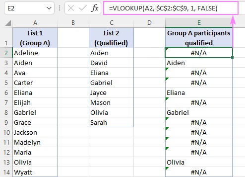
2.3. Interpreting the Results

If a value from List 1 is found in List 2, the VLOOKUP formula will return that value in the result column.
If a value from List 1 is not found in List 2, the VLOOKUP formula will return a #N/A error.

3. Handling #N/A Errors

The #N/A error can be unsightly and confusing. To handle these errors and make your results more user-friendly, you can use the IFNA or IFERROR functions in combination with VLOOKUP.

3.1. Using IFNA

The IFNA function allows you to replace #N/A errors with a specified value. The syntax is:

=IFNA(value, value_if_na)

value: The expression to evaluate (in this case, the VLOOKUP formula).
value_if_na: The value to return if the value argument results in a #N/A error.

To replace #N/A errors with blank cells, modify the VLOOKUP formula as follows:

=IFNA(VLOOKUP(A2, $C$2:$C$10, 1, FALSE), "")

This formula will return the matching value if found, and a blank cell if not found.

To return custom text, such as “Not Found,” use the following formula:

=IFNA(VLOOKUP(A2, $C$2:$C$10, 1, FALSE), "Not Found")

3.2. Using IFERROR

The IFERROR function is similar to IFNA, but it catches all types of errors, not just #N/A errors. The syntax is:

=IFERROR(value, value_if_error)

To use IFERROR to handle #N/A errors, modify the VLOOKUP formula as follows:

=IFERROR(VLOOKUP(A2, $C$2:$C$10, 1, FALSE), "")

4. Comparing Two Columns in Different Excel Sheets

In real-world scenarios, the columns you want to compare may reside in different worksheets within the same or different Excel files. To compare columns across sheets, you need to use external references in your VLOOKUP formula.

4.1. Referencing Columns in Another Sheet

Assume List 1 is in Column A of “Sheet1” and List 2 is in Column A of “Sheet2.” To compare the columns and find matches, use the following formula in Sheet1:

=IFNA(VLOOKUP(A2, Sheet2!$A$2:$A$10, 1, FALSE), "")

The “Sheet2!$A$2:$A$10” part of the formula is an external reference that points to the range of cells containing List 2 in Sheet2.

4.2. Referencing Columns in Another Workbook

To compare columns in different workbooks, you need to include the workbook name in the external reference. For example, if List 2 is in Column A of “Sheet1” in a workbook named “Data.xlsx,” the formula would be:

=IFNA(VLOOKUP(A2, '[Data.xlsx]Sheet1'!$A$2:$A$10, 1, FALSE), "")

Note: When referencing another workbook, the workbook must be open for the formula to work correctly.

5. Returning Common Values (Matches)

The basic VLOOKUP formula returns a list of values that exist in both columns, along with blank cells or custom text for missing values. To extract a list of only the common values without gaps, you can use filtering or dynamic array formulas.

5.1. Using Filtering

Apply the VLOOKUP formula: Use the basic VLOOKUP formula with IFNA or IFERROR to generate the result column.
Apply AutoFilter: Select the result column and go to the “Data” tab in the Excel ribbon. Click on the “Filter” button.
Filter out blanks: Click the filter arrow in the result column header and uncheck the “Blanks” option. This will display only the common values.

5.2. Using Dynamic Array Formulas (Excel 365 and Excel 2021)

Excel 365 and Excel 2021 support dynamic arrays, which allow formulas to return multiple values automatically. You can use the FILTER function in combination with VLOOKUP to extract common values dynamically.

=FILTER(A2:A10, IFNA(VLOOKUP(A2:A10, C2:C10, 1, FALSE), "")<>"")

This formula compares each value in List 1 (A2:A10) against List 2 (C2:C10) and returns an array of matches. The IFNA function replaces errors with empty strings, and the FILTER function filters out blanks, outputting only the common values.

Alternatively, you can use the ISNA function:

=FILTER(A2:A10, ISNA(VLOOKUP(A2:A10, C2:C10, 1, FALSE))=FALSE)

Or, with XLOOKUP:

=FILTER(A2:A10, XLOOKUP(A2:A10, C2:C10, C2:C10,"")<>"")

6. Finding Missing Values (Differences)

To find values that exist in one column but not the other, you can modify the VLOOKUP formula to identify differences.

6.1. Identifying Missing Values in List 2

To find values in List 1 that are not present in List 2, use the following formula:

=IF(ISNA(VLOOKUP(A2, $C$2:$C$10, 1, FALSE)), A2, "")

This formula checks if the VLOOKUP returns a #N/A error (meaning the value is not found in List 2). If it does, the formula returns the value from List 1; otherwise, it returns a blank cell.

To filter out the blanks and display only the missing values, use Excel’s Filter as described earlier.

6.2. Using Dynamic Array Formulas for Missing Values

In Excel 365 and Excel 2021, you can use the FILTER function to dynamically extract missing values:

=FILTER(A2:A10, ISNA(VLOOKUP(A2:A10, C2:C10, 1, FALSE)))

This formula filters List 1 based on whether the values are not found in List 2, returning only the missing values.

Alternatively, using XLOOKUP:

=FILTER(A2:A10, XLOOKUP(A2:A10, C2:C10, C2:C10,"")="")

7. Identifying Matches and Differences with Text Labels

To add text labels indicating whether a value is a match or a difference, you can combine VLOOKUP with the IF and ISNA/ISERROR functions.

=IF(ISNA(VLOOKUP(A2, $D$2:$D$10, 1, FALSE)), "Not in List 2", "In List 2")

This formula checks if a value from List 1 (Column A) is found in List 2 (Column D). If it is, the formula returns “In List 2”; otherwise, it returns “Not in List 2.”

Alternatively, using the MATCH function:

=IF(ISNA(MATCH(A2, $D$2:$D$10, 0)), "Not in List 2", "In List 2")

8. Returning a Value from a Third Column Based on the Comparison

One of the most powerful applications of VLOOKUP is to compare two columns and return a corresponding value from a third column. This is particularly useful when working with tables containing related data.

Suppose you have two tables: one with a list of names and another with a list of names and their corresponding scores. You want to compare the names in the two tables and return the score for each matching name.

=VLOOKUP(A2, $D$2:$E$10, 2, FALSE)

A2: The name you want to search for in the second table.
$D$2:$E$10: The range of cells containing the second table, with names in Column D and scores in Column E.
2: The column number within the table_array to return a value from (Column E, containing the scores).
FALSE: Specifies that we want an exact match.

To handle #N/A errors, use the IFNA function:

=IFNA(VLOOKUP(A2, $D$2:$E$10, 2, FALSE), "Not Available")

This formula will return the score for matching names and “Not Available” for names not found in the second table.

Instead of VLOOKUP, you can use INDEX MATCH:

=IFNA(INDEX($E$2:$E$10, MATCH(A2, $D$2:$D$10, 0)), "Not Available")

Or XLOOKUP:

=XLOOKUP(A2, $D$2:$D$10, $E$2:$E$10, "Not Available")

9. Alternatives to VLOOKUP

While VLOOKUP is a valuable tool, Excel offers other functions that can be used for column comparison, each with its own strengths and weaknesses.

9.1. MATCH

The MATCH function searches for a value in a range of cells and returns the relative position of that value in the range. It can be used to check if a value exists in a column.

=IF(ISNA(MATCH(A2, $C$2:$C$10, 0)), "Not Found", "Found")

9.2. INDEX MATCH

The INDEX MATCH combination is a more flexible alternative to VLOOKUP. INDEX returns a value from a specified row and column in a range, while MATCH returns the position of a value in a range. Together, they can perform more complex lookups.

=INDEX($E$2:$E$10, MATCH(A2, $D$2:$D$10, 0))

9.3. XLOOKUP

XLOOKUP is a modern successor to VLOOKUP, available in Excel 365 and Excel 2021. It offers several advantages over VLOOKUP, including better handling of errors, the ability to search in both directions, and simpler syntax.

=XLOOKUP(A2, $D$2:$D$10, $E$2:$E$10, "Not Found")

10. Best Practices for Using VLOOKUP

To ensure accurate and efficient column comparison using VLOOKUP, follow these best practices:

Use Absolute References: Always use absolute references ($) for the table_array argument to prevent the range from changing when you copy the formula.
Ensure Exact Matches: Use FALSE for the range_lookup argument to ensure you’re performing exact match comparisons.
Handle Errors: Use IFNA or IFERROR to handle #N/A errors and provide user-friendly results.
Sort Data: If you’re using approximate match (TRUE for range_lookup), make sure the first column of the table_array is sorted in ascending order.
Consider Alternatives: Explore other lookup functions like MATCH, INDEX MATCH, and XLOOKUP to see if they better suit your needs.
Keep it Simple: Break down complex comparisons into smaller, more manageable formulas.
Test Thoroughly: Always test your VLOOKUP formulas to ensure they’re returning the correct results.

11. Real-World Applications

Comparing two columns in Excel using VLOOKUP has numerous real-world applications across various industries:

Data Validation: Ensuring data consistency between two datasets.
Reconciliation: Identifying discrepancies between financial records.
Inventory Management: Comparing stock levels across different locations.
Customer Relationship Management (CRM): Identifying duplicate customer records.
Human Resources: Comparing employee lists and identifying missing information.

12. Potential Issues and Troubleshooting

While VLOOKUP is a powerful tool, you may encounter some issues when using it. Here are some common problems and how to troubleshoot them:

#N/A Errors: These errors indicate that the lookup_value was not found in the table_array. Double-check that the values you’re searching for exist in the correct column and that the range_lookup argument is set correctly.
Incorrect Results: If VLOOKUP returns the wrong value, ensure that the col_index_num argument is correct and that the table_array is properly defined.
Performance Issues: When working with large datasets, VLOOKUP can be slow. Consider using alternative functions or optimizing your data.
Case Sensitivity: VLOOKUP is not case-sensitive. If you need to perform a case-sensitive comparison, use a different approach, such as combining the EXACT function with array formulas.

13. Automating Column Comparison

For repetitive column comparison tasks, you can automate the process using Excel VBA (Visual Basic for Applications). VBA allows you to write custom code to perform complex operations, such as comparing columns, extracting data, and generating reports.

13.1. VBA Example: Comparing Two Columns and Returning Matches

The following VBA code compares two columns in a worksheet and returns the matching values in a third column:

Sub CompareColumns()

  Dim ws As Worksheet
  Dim lastRow1 As Long, lastRow2 As Long
  Dim i As Long, j As Long
  Dim matchFound As Boolean

  Set ws = ThisWorkbook.Sheets("Sheet1") ' Replace "Sheet1" with your sheet name

  lastRow1 = ws.Cells(Rows.Count, "A").End(xlUp).Row ' Last row in Column A
  lastRow2 = ws.Cells(Rows.Count, "C").End(xlUp).Row ' Last row in Column C

  j = 2 ' Start writing matches in Column E from row 2

  For i = 2 To lastRow1 ' Loop through Column A
    matchFound = False
    For k = 2 To lastRow2 ' Loop through Column C
      If ws.Cells(i, "A").Value = ws.Cells(k, "C").Value Then
        matchFound = True
        Exit For
      End If
    Next k

    If matchFound Then
      ws.Cells(j, "E").Value = ws.Cells(i, "A").Value ' Write match to Column E
      j = j + 1
    End If
  Next i

  MsgBox "Column comparison complete!"

End Sub

This code iterates through each value in Column A and checks if it exists in Column C. If a match is found, the value is written to Column E.

13.2. Running the VBA Code

Open the VBA editor in Excel (Alt + F11).
Insert a new module (Insert > Module).
Copy and paste the VBA code into the module.
Modify the sheet name and column references as needed.
Run the code by pressing F5 or clicking the “Run” button.

14. Advanced Techniques

For more advanced column comparison scenarios, you can explore techniques such as:

Conditional Formatting: Use conditional formatting to highlight matching or missing values in columns.
Array Formulas: Use array formulas to perform complex comparisons and calculations on entire ranges of cells.
Power Query: Use Power Query to import and transform data from multiple sources and perform advanced data analysis.

15. Conclusion

Comparing two columns in Excel using VLOOKUP is a fundamental skill for data analysis and validation. By understanding the principles of VLOOKUP and its variations, you can efficiently extract valuable insights from your data. Whether you’re identifying common values, finding missing information, or returning related data, VLOOKUP empowers you to make informed decisions.

Visit COMPARE.EDU.VN for more resources and tutorials on Excel and other data analysis tools. With the right knowledge and techniques, you can unlock the full potential of Excel and gain a competitive edge in your field.

Do you find yourself struggling to compare complex datasets? Are you tired of manually searching for differences and matches? Visit COMPARE.EDU.VN today and discover a world of efficient comparison tools and techniques. Let us help you make smarter decisions, faster. Contact us at 333 Comparison Plaza, Choice City, CA 90210, United States or Whatsapp: +1 (626) 555-9090. COMPARE.EDU.VN – Your trusted partner in informed decision-making.

16. FAQ

Q1: Can VLOOKUP compare columns with different data types?

A: VLOOKUP works best when comparing columns with the same data types. If you’re comparing columns with different data types, you may need to convert the data types using functions like TEXT, VALUE, or DATE.

Q2: How can I compare two columns case-sensitively using VLOOKUP?

A: VLOOKUP is not case-sensitive. To perform a case-sensitive comparison, you can use the EXACT function in combination with array formulas.

Q3: Can VLOOKUP compare columns in different Excel files?

A: Yes, you can compare columns in different Excel files by using external references in your VLOOKUP formula.

Q4: What are the limitations of VLOOKUP when comparing large datasets?

A: VLOOKUP can be slow when comparing large datasets. Consider using alternative functions like INDEX MATCH or XLOOKUP, or optimizing your data by sorting it or using helper columns.

Q5: How can I handle errors when using VLOOKUP?

A: You can use the IFNA or IFERROR functions to handle errors and provide user-friendly results.

Q6: Can VLOOKUP return multiple values based on a single lookup value?

A: VLOOKUP can only return one value for each lookup value. To return multiple values, you can use alternative functions like INDEX MATCH with multiple criteria or Power Query.

Q7: Is VLOOKUP the best function for comparing two columns in Excel?

A: VLOOKUP is a useful function, but it’s not always the best choice. Depending on your specific needs, you may find that other functions like MATCH, INDEX MATCH, or XLOOKUP are more suitable.

Q8: How can I automate column comparison in Excel?

A: You can automate column comparison in Excel using VBA (Visual Basic for Applications). VBA allows you to write custom code to perform complex operations and generate reports.

Q9: What are some advanced techniques for column comparison in Excel?

A: Some advanced techniques for column comparison include using conditional formatting, array formulas, and Power Query.

Q10: Where can I find more resources and tutorials on Excel and data analysis?

A: You can find more resources and tutorials on Excel and data analysis at compare.edu.vn and other reputable websites and online courses.