How To Compare Two Columns On Different Sheets In Excel?

Are you looking for ways on How To Compare Two Columns On Different Sheets In Excel to identify discrepancies and ensure data integrity? At COMPARE.EDU.VN, we provide a comprehensive guide to help you master this essential skill. By using techniques ranging from simple formulas to conditional formatting, you can identify, highlight, and manage differences effectively. This guide helps you make informed decisions based on accurate data analysis and informed comparison. Explore our resources for effective data comparison and data validation in Excel.

1. What Is The Easiest Way To Compare Two Columns In Excel?

The easiest way to compare two columns in Excel is by using a simple formula. This method quickly highlights differences between corresponding cells in two columns, making it ideal for identifying discrepancies in datasets.

Here’s how to do it:

Open your Excel workbook: Make sure the two columns you want to compare are in different sheets within the same workbook.
Create a new column: In a third sheet, create a new column next to the columns you want to compare. This column will display the comparison results.
Enter the formula: In the first cell of the new column, enter the following formula:

=IF(Sheet1!A1=Sheet2!A1, "Match", "Mismatch")
- Replace Sheet1 and Sheet2 with the actual names of your sheets.
- Replace A1 with the first cell in the columns you want to compare.
Copy the formula: Drag the fill handle (the small square at the bottom-right of the cell) down to apply the formula to all the rows you want to compare.

This formula compares the values in the corresponding cells of the two columns. If the values are the same, it displays “Match”; otherwise, it displays “Mismatch”.
Filter the results (Optional): If you want to quickly see only the mismatches, you can filter the column with the formula. Select the column, go to the “Data” tab, click “Filter,” and then filter the column to show only the “Mismatch” results.

By following these steps, you can quickly compare two columns in Excel and identify any differences between them. This method is straightforward and requires no advanced Excel skills.

2. How Can I Use Conditional Formatting To Compare Two Columns In Excel?

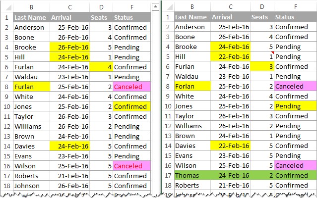
Conditional formatting is a powerful tool in Excel that allows you to automatically format cells based on certain criteria. Using conditional formatting to compare two columns can visually highlight differences, making it easier to identify discrepancies at a glance.

Here’s how to use conditional formatting for this purpose:

Select the range: Choose the column or range of cells in the first sheet that you want to compare. This is the column where the formatting will be applied.
Open Conditional Formatting: Go to the “Home” tab in the Excel ribbon, click on “Conditional Formatting” in the “Styles” group, and select “New Rule”.
Create a New Rule: In the “New Formatting Rule” dialog box, select “Use a formula to determine which cells to format”.
Enter the formula: Enter the following formula in the formula box:

=A1<>Sheet2!A1
- Replace A1 with the first cell in the selected range in your first sheet.
- Replace Sheet2 with the name of the second sheet.
- Replace A1 after Sheet2! with the corresponding first cell in the second sheet that you are comparing.
This formula checks if the value in the current cell of the first sheet is different from the value in the corresponding cell of the second sheet.
Set the Format: Click the “Format” button to set the formatting style that will be applied to the cells where the values are different. You can change the font, border, fill color, etc. For example, you might choose to fill the cell with a bright color like red or yellow to make the differences stand out.
Apply the Rule: Click “OK” to close the “Format Cells” dialog box, and then click “OK” again to close the “New Formatting Rule” dialog box.
Check the results: Excel will now highlight all the cells in the selected range that have different values compared to the corresponding cells in the second sheet.

By using conditional formatting in this way, you can easily spot any discrepancies between the two columns. This method is particularly useful for large datasets where manual comparison would be time-consuming and prone to error.

3. How To Compare Data From Two Excel Sheets And Create A Report?

To compare data from two Excel sheets and create a report, you can use a combination of formulas and Excel’s reporting features. This approach allows you to not only identify differences but also present them in a structured and easily understandable format.

Here’s how to do it:

Set up your sheets: Ensure that both sheets contain the data you want to compare. The sheets should have a similar structure, with corresponding data in the same columns.
Create a new report sheet: Add a new sheet to your Excel workbook. This sheet will be used to generate the comparison report.
Add headers to the report sheet: In the report sheet, add headers that correspond to the columns you are comparing. Also, add a column for the comparison result (e.g., “Status”).
Enter the comparison formula: In the first data row of the report sheet, enter a formula to compare the corresponding cells in the two source sheets. For example, if you are comparing column A in Sheet1 and Sheet2, the formula in the “Status” column of the report sheet would be:

=IF(Sheet1!A2=Sheet2!A2, "Match", "Mismatch")
- Sheet1 and Sheet2 are the names of your source sheets.
- A2 is the first data cell in column A of both sheets.
Copy the formula down: Drag the fill handle (the small square at the bottom-right of the cell) down to apply the formula to all the rows you want to compare.
Add data from the source sheets: In the report sheet, add formulas to pull the data from the source sheets. For example, in column A of the report sheet, you would enter =Sheet1!A2 to pull data from Sheet1, and in column B, you would enter =Sheet2!A2 to pull data from Sheet2. Adjust the cell references as necessary.
Use Conditional Formatting: Apply conditional formatting to the “Status” column to highlight the “Mismatch” results. This will make it easier to visually identify the differences.
Create a summary: At the top or bottom of the report sheet, create a summary section that counts the number of matches and mismatches. You can use the COUNTIF function for this:
- To count the number of matches, use: =COUNTIF(StatusColumn, "Match")
- To count the number of mismatches, use: =COUNTIF(StatusColumn, "Mismatch")
Replace StatusColumn with the range of cells in your “Status” column (e.g., E2:E100).
Format the report: Apply formatting to the report sheet to make it more readable. Use borders, colors, and appropriate font sizes to highlight the key information.

By following these steps, you can create a detailed comparison report that not only identifies the differences between two Excel sheets but also presents the data in an organized and informative manner. This type of report is invaluable for data validation, auditing, and reconciliation tasks.

4. What Excel Functions Are Useful For Comparing Columns?

Excel offers a variety of functions that are useful for comparing columns and identifying differences or similarities between them. These functions can help you perform simple comparisons, find matching values, or identify unique entries. Here are some of the most useful Excel functions for comparing columns:

IF: The IF function is one of the most basic and versatile functions for comparing columns. It allows you to specify a condition and return different values based on whether the condition is true or false.
- Example: =IF(A1=B1, "Match", "Mismatch") compares the values in cells A1 and B1 and returns “Match” if they are the same, and “Mismatch” if they are different.
EXACT: The EXACT function compares two text strings and returns TRUE if they are exactly the same (case-sensitive), and FALSE otherwise.
- Example: =EXACT(A1, B1) compares the text in cells A1 and B1 and returns TRUE only if they are identical, including capitalization.
VLOOKUP: The VLOOKUP function is used to find a value in one column and return a corresponding value from another column in the same row. It’s particularly useful for comparing a column against a reference table to find matches.
- Example: =VLOOKUP(A1, Sheet2!A:B, 2, FALSE) looks for the value in A1 of the current sheet in column A of Sheet2. If it finds a match, it returns the value from column B of Sheet2 in the same row. The FALSE argument ensures an exact match.
MATCH: The MATCH function searches for a specified item in a range of cells and returns the relative position of that item in the range. It can be used to determine if a value in one column exists in another column.
- Example: =ISNUMBER(MATCH(A1, B:B, 0)) checks if the value in A1 exists in column B. The MATCH function returns the position if found, and the ISNUMBER function converts this to TRUE. If not found, MATCH returns an error, and ISNUMBER returns FALSE.
COUNTIF: The COUNTIF function counts the number of cells within a range that meet a given criteria. It can be used to determine how many times a value from one column appears in another column.
- Example: =COUNTIF(B:B, A1) counts how many times the value in A1 appears in column B. A result greater than 0 indicates that the value exists in column B.
ISNA: The ISNA function checks whether a value is #N/A (Not Available). It’s often used in conjunction with VLOOKUP or MATCH to handle cases where a value is not found.
- Example: =ISNA(VLOOKUP(A1, Sheet2!A:B, 2, FALSE)) checks if the VLOOKUP function returns an #N/A error, indicating that the value in A1 was not found in column A of Sheet2.
SUMPRODUCT: The SUMPRODUCT function multiplies corresponding components in the given arrays and returns the sum of those products. It can be used for more complex comparisons involving multiple criteria.
- Example: =SUMPRODUCT(--(A1:A10=B1:B10)) compares the ranges A1:A10 and B1:B10. The double negative (--) converts the TRUE/FALSE results of the comparison into 1s and 0s, which SUMPRODUCT then sums. The result is the number of rows where the values in the two ranges are equal.

By using these Excel functions, you can perform a wide range of column comparisons to identify matches, mismatches, and other relevant data patterns, enhancing your data analysis capabilities.

5. How Can I Highlight Duplicate Values Across Two Columns?

Highlighting duplicate values across two columns in Excel is a useful technique for identifying common entries and ensuring data consistency. Excel’s conditional formatting feature makes this task straightforward.

Here’s how to highlight duplicate values across two columns:

Select both columns: Click and drag to select both columns that you want to compare for duplicate values.
Open Conditional Formatting: Go to the “Home” tab on the Excel ribbon. In the “Styles” group, click on “Conditional Formatting”.
Choose Highlight Cells Rule: From the dropdown menu, select “Highlight Cells Rules” and then choose “Duplicate Values”.
Set the formatting: In the “Duplicate Values” dialog box, you can choose how you want the duplicate values to be highlighted. By default, Excel will format duplicate values with a light red fill and dark red text. You can change this by selecting a different formatting option from the dropdown menu (e.g., yellow fill, green fill, or custom format).
Apply the rule: Click “OK” to apply the conditional formatting rule.
Review the results: Excel will now highlight all the values that appear in both columns. These are the duplicate values that are common to both columns.

By following these steps, you can quickly and easily highlight duplicate values across two columns in Excel. This method is useful for tasks such as identifying common customers in two lists, finding overlapping products in inventory databases, or detecting redundant entries in any type of dataset.

6. How Do I Compare Two Columns For Similar Text And Find Partial Matches?

Comparing two columns for similar text and finding partial matches can be more complex than simple exact match comparisons. This task often requires using formulas that can identify if one text string is contained within another. Here’s how you can achieve this in Excel:

Set up your sheets: Ensure that both sheets contain the data you want to compare. The sheets should have a similar structure, with corresponding data in the same columns.
Use the SEARCH function: The SEARCH function finds one text string within another and returns the position of the first text string. If the first text string is not found, it returns an error. We can use this to check for partial matches.
Combine with ISNUMBER: The ISNUMBER function checks whether a value is a number. When combined with SEARCH, it can tell us if the text was found (resulting in a number) or not (resulting in an error, which ISNUMBER will evaluate as FALSE).
Enter the formula: In a third column, enter the following formula:

=IF(ISNUMBER(SEARCH(Sheet1!A1, Sheet2!B1)), "Partial Match", "No Match")
- Sheet1!A1 is the cell containing the text you want to search for.
- Sheet2!B1 is the cell containing the text you want to search within.
Copy the formula: Drag the fill handle (the small square at the bottom-right of the cell) down to apply the formula to all the rows you want to compare.
Review the results: The formula will return “Partial Match” if the text in Sheet1!A1 is found within the text in Sheet2!B1, and “No Match” if it is not found.
Refine the results with additional criteria (Optional): If needed, you can add additional criteria to the formula to refine the matching process. For example, you might want to check the length of the matched text or ensure that certain keywords are present.

By following these steps, you can compare two columns for similar text and find partial matches in Excel. This technique is useful for tasks such as identifying related product names, matching customer addresses, or detecting similar phrases in text documents.

7. How Can Excel VBA Be Used To Compare Two Columns?

Excel VBA (Visual Basic for Applications) can be used to compare two columns, providing a powerful and flexible way to automate the comparison process, especially for complex scenarios.

Here’s how you can use VBA to compare two columns:

Open the VBA Editor: Press Alt + F11 to open the VBA editor in Excel.
Insert a New Module: In the VBA editor, go to “Insert” > “Module”. This is where you will write your VBA code.
Write the VBA Code: Copy and paste the following VBA code into the module:

Sub CompareColumns()

    Dim ws1 As Worksheet, ws2 As Worksheet
    Dim lastRow As Long, i As Long
    Dim col1 As Range, col2 As Range
    Dim cell1 As Range, cell2 As Range

    ' Set the worksheet names
    Set ws1 = ThisWorkbook.Sheets("Sheet1")
    Set ws2 = ThisWorkbook.Sheets("Sheet2")

    ' Set the columns to compare
    Set col1 = ws1.Range("A:A")
    Set col2 = ws2.Range("A:A")

    ' Find the last row with data in both columns
    lastRow = Application.WorksheetFunction.Max(ws1.Cells(Rows.Count, "A").End(xlUp).Row, _
                                                 ws2.Cells(Rows.Count, "A").End(xlUp).Row)

    ' Loop through each row and compare the values
    For i = 1 To lastRow
        Set cell1 = ws1.Cells(i, "A")
        Set cell2 = ws2.Cells(i, "A")

        If cell1.Value <> cell2.Value Then
            ' Highlight the differences
            cell1.Interior.Color = RGB(255, 0, 0) ' Red
            cell2.Interior.Color = RGB(255, 0, 0) ' Red
        End If
    Next i

    MsgBox "Comparison complete. Differences highlighted in red."

End Sub

Modify the Code (if needed):
- Change the worksheet names (“Sheet1” and “Sheet2”) to match the names of your sheets.
- Modify the column ranges (“A:A”) to match the columns you want to compare.
- Adjust the highlighting color (RGB values) as desired.
Run the Macro: Close the VBA editor and go back to your Excel sheet. Go to the “Developer” tab and click on “Macros”. Select the “CompareColumns” macro and click “Run”. If you don’t see the “Developer” tab, you may need to enable it in Excel’s options.
Review the Results: The macro will compare the values in the specified columns and highlight any differences in red.

By using VBA, you can create custom comparison scripts that handle complex scenarios, such as ignoring case, trimming spaces, or performing partial matches. This level of automation is invaluable for large datasets and recurring comparison tasks.

8. How Can I Ignore Case When Comparing Two Columns In Excel?

Ignoring case when comparing two columns in Excel ensures that text comparisons are not case-sensitive, treating “Apple” and “apple” as the same. This can be achieved using the UPPER or LOWER functions in combination with the IF function.

Here’s how to ignore case when comparing two columns:

Open your Excel workbook: Make sure the two columns you want to compare are in different sheets within the same workbook.
Create a new column: In a third sheet, create a new column next to the columns you want to compare. This column will display the comparison results.
Enter the formula: In the first cell of the new column, enter the following formula:

=IF(UPPER(Sheet1!A1)=UPPER(Sheet2!A1), "Match", "Mismatch")

Replace Sheet1 and Sheet2 with the actual names of your sheets.
Replace A1 with the first cell in the columns you want to compare.

Copy the formula: Drag the fill handle (the small square at the bottom-right of the cell) down to apply the formula to all the rows you want to compare.

This formula compares the values in the corresponding cells of the two columns. If the values are the same, it displays “Match”; otherwise, it displays “Mismatch”.

Filter the results (Optional): If you want to quickly see only the mismatches, you can filter the column with the formula. Select the column, go to the “Data” tab, click “Filter,” and then filter the column to show only the “Mismatch” results.

By following these steps, you can quickly compare two columns in Excel and identify any differences between them. This method is straightforward and requires no advanced Excel skills.

9. Is There A Way To Compare Only Specific Rows In Two Columns?

Yes, there is a way to compare only specific rows in two columns in Excel. This can be achieved by adjusting the formulas or VBA code to reference only the specific rows you want to compare. Here are a few methods to accomplish this:

Using Formulas with Specific Cell References:

If you want to compare only a few specific rows, you can directly reference those cells in your formula.
- Example: To compare only rows 3, 5, and 7 of column A in Sheet1 with column A in Sheet2, you would create separate comparison formulas for each row:
  
  =IF(Sheet1!A3=Sheet2!A3, "Match", "Mismatch")
  
  =IF(Sheet1!A5=Sheet2!A5, "Match", "Mismatch")
  
  =IF(Sheet1!A7=Sheet2!A7, "Match", "Mismatch")
This method is suitable when you have a small, fixed number of rows to compare.
Using Named Ranges and Formulas:

You can define named ranges for the specific rows you want to compare and then use those ranges in your formulas.
- Select the specific cells in Sheet1 (e.g., A3, A5, A7) and go to the “Formulas” tab, click “Define Name”, and give it a name (e.g., SpecificRows1).
- Do the same for the corresponding cells in Sheet2 (e.g., A3, A5, A7) and name it SpecificRows2.
- In a third column, use the following formula:
  
  =IF(INDEX(SpecificRows1, ROW()-ROW(FirstCell)+1) = INDEX(SpecificRows2, ROW()-ROW(FirstCell)+1), "Match", "Mismatch")
  
  Replace FirstCell with the first cell where you enter this formula. This formula will dynamically compare the corresponding rows in the named ranges.

Using VBA with Specific Row Numbers:

You can write a VBA macro that loops through only the specific row numbers you want to compare.

Open the VBA editor (Alt + F11).
Insert a new module (“Insert” > “Module”).
Copy and paste the following VBA code:

Sub CompareSpecificRows()
    Dim ws1 As Worksheet, ws2 As Worksheet
    Dim rowNumbers As Variant, i As Long
    Dim cell1 As Range, cell2 As Range

    ' Set the worksheet names
    Set ws1 = ThisWorkbook.Sheets("Sheet1")
    Set ws2 = ThisWorkbook.Sheets("Sheet2")

    ' Define the specific row numbers to compare
    rowNumbers = Array(3, 5, 7)

    ' Loop through each specified row and compare the values
    For i = LBound(rowNumbers) To UBound(rowNumbers)
        Set cell1 = ws1.Cells(rowNumbers(i), "A")
        Set cell2 = ws2.Cells(rowNumbers(i), "A")

        If cell1.Value <> cell2.Value Then
            ' Highlight the differences
            cell1.Interior.Color = RGB(255, 0, 0) ' Red
            cell2.Interior.Color = RGB(255, 0, 0) ' Red
        End If
    Next i

    MsgBox "Comparison complete. Differences highlighted in red."
End Sub

Modify the code to specify the worksheet names and the row numbers you want to compare.
Run the macro.

This VBA macro will compare only the specified rows and highlight any differences.

By using these methods, you can efficiently compare only the specific rows you need to analyze, saving time and focusing your comparison efforts.

10. How Do I Display Only The Differences Between Two Columns In Excel?

Displaying only the differences between two columns in Excel involves first identifying the differences and then filtering the results to show only those rows where differences exist. This can be achieved using a combination of formulas and Excel’s filtering capabilities.

Here’s how to display only the differences between two columns:

Set up your sheets: Ensure that both sheets contain the data you want to compare. The sheets should have a similar structure, with corresponding data in the same columns.
Create a new column: In a third sheet, create a new column next to the columns you want to compare. This column will display the comparison results.
Enter the comparison formula: In the first cell of the new column, enter the following formula:

=IF(Sheet1!A1=Sheet2!A1, "Match", "Mismatch")
- Replace Sheet1 and Sheet2 with the actual names of your sheets.
- Replace A1 with the first cell in the columns you want to compare.
Copy the formula: Drag the fill handle (the small square at the bottom-right of the cell) down to apply the formula to all the rows you want to compare.
Apply the Filter:
- Select the range of cells that includes your data and the comparison results.
- Go to the “Data” tab on the Excel ribbon.
- Click the “Filter” button. This will add dropdown arrows to the headers of your columns.
Filter the “Status” column:
- Click the dropdown arrow in the header of the “Status” column (the column with the “Match” and “Mismatch” results).
- Uncheck the “Select All” box to clear all selections.
- Check the “Mismatch” box to select only the rows where there are differences.
- Click “OK”.
Review the results: Excel will now display only the rows where the values in the two compared columns are different.

By following these steps, you can quickly and easily display only the differences between two columns in Excel. This method is useful for focusing on discrepancies, identifying errors, and performing targeted data analysis.

Navigating the complexities of data comparison in Excel doesn’t have to be a daunting task. With the right techniques, you can efficiently identify differences, highlight discrepancies, and create detailed reports that streamline your data analysis process. Whether you’re using simple formulas, conditional formatting, or VBA, the methods outlined in this guide will empower you to make informed decisions based on accurate data.

Ready to Take Your Excel Skills to the Next Level?

At COMPARE.EDU.VN, we understand the challenges you face when comparing data. That’s why we offer comprehensive guides and resources to help you master Excel and other essential tools.

Here’s how we can help:

Detailed Comparisons: Access in-depth comparisons of various products, services, and tools to make informed decisions.
Step-by-Step Tutorials: Learn practical skills with our easy-to-follow guides.
Expert Reviews: Get insights from industry experts to ensure you’re using the best solutions.

Visit COMPARE.EDU.VN today to discover more and unlock your full potential!

Address: 333 Comparison Plaza, Choice City, CA 90210, United States

WhatsApp: +1 (626) 555-9090

Website: compare.edu.vn

FAQ: Comparing Columns in Excel

How do I compare two columns in Excel and highlight the differences?
- Use conditional formatting with a formula like =A1<>Sheet2!A1 to highlight different cells.
Can I compare two columns for partial matches in Excel?
- Yes, use the SEARCH function combined with ISNUMBER in a formula like =IF(ISNUMBER(SEARCH(Sheet1!A1, Sheet2!B1)), "Partial Match", "No Match").
How do I ignore case when comparing two columns in Excel?
- Use the UPPER or LOWER functions in your comparison formula, such as =IF(UPPER(A1)=UPPER(B1), "Match", "Mismatch").
Is it possible to compare only specific rows in two columns?
- Yes, reference specific cells directly in your formulas or use VBA to loop through specific row numbers.
How can I display only the differences between two columns in Excel?
- Use a comparison formula to identify differences and then apply a filter to show only the “Mismatch” results.
What Excel functions are useful for comparing columns?
- IF, EXACT, VLOOKUP, MATCH, COUNTIF, ISNA, and SUMPRODUCT are all useful functions for comparing columns.
How do I compare data from two Excel sheets and create a report?
- Create a new sheet with comparison formulas, pull data from the source sheets, and use conditional formatting to highlight differences.
Can I use Excel VBA to compare two columns?
- Yes, VBA can automate complex comparison scenarios, such as ignoring case, trimming spaces, or performing partial matches.
How do I highlight duplicate values across two columns in Excel?
- Use conditional formatting with the “Duplicate Values” rule to highlight common entries.
How can I create a case-sensitive comparison in Excel?
- Use the EXACT function, which returns TRUE only if two text strings are exactly the same, including capitalization.