**How To Compare Two Columns In Excel With Formula?**

Comparing two columns in Excel with a formula is a common task that helps identify matching or differing data, and COMPARE.EDU.VN offers comprehensive guides to streamline this process. By using formulas and conditional formatting, you can highlight duplicates, find unique values, and ensure data consistency. Leverage comparison techniques and data analysis tools for efficient Excel use.

1. Why Is Comparing Two Columns in Excel Useful?

Comparing two columns in Excel is a crucial skill for data analysis, data validation, and ensuring data integrity. Excel’s ability to compare data across columns is essential for data analysts to make informed decisions. Manually comparing columns can be time-consuming and prone to errors, especially when dealing with large datasets.

1.1 Data Validation

Data validation involves ensuring that data entered into a system or database is accurate and conforms to predefined rules and constraints. Comparing columns allows you to verify the accuracy of data entry and identify discrepancies. For example, you can compare a list of customer IDs against a master list to ensure all entries are valid.

1.2 Data Analysis

Data analysis involves inspecting, cleansing, transforming, and modeling data to discover useful information, draw conclusions, and support decision-making. Comparing columns allows you to identify patterns, trends, and relationships within the data. For instance, you can compare sales data from two different periods to identify growth areas.

1.3 Data Cleansing

Data cleansing is the process of detecting and correcting (or removing) corrupt or inaccurate records from a record set, table, or database. Comparing columns helps you identify and correct inconsistencies in your data, such as duplicate entries or mismatched values. For example, you can compare two lists of email addresses to remove duplicates.

2. What Are the Methods to Compare Two Columns in Excel?

There are several methods to compare two columns in Excel, each with its own strengths and applications. These methods include using the equals operator, IF condition, EXACT function, conditional formatting, and lookup functions.

2.1 Using the Equals Operator

The equals operator (=) is a simple way to compare two columns row by row. This method returns TRUE if the values in the compared columns are the same and FALSE if they differ.

Example

To use the equals operator, enter the formula =A1=B1 in a cell (e.g., C1). Drag this formula down to apply it to all rows in the columns you want to compare. The result will be a column of TRUE and FALSE values, indicating whether the corresponding rows match.

2.2 Using the IF Condition

The IF condition allows you to return custom results, such as “Match” or “Not Match,” based on whether the values in two columns are equal.

Example

To use the IF condition, enter the formula =IF(A1=B1, "Match", "Not Match") in a cell (e.g., C1). Drag this formula down to apply it to all rows. The result will be a column displaying “Match” for rows where the values are the same and “Not Match” where they differ.

2.3 Using the EXACT Function

The EXACT function is case-sensitive and ensures that the values in two columns are identical, including capitalization. This is particularly useful when comparing text strings where case matters.

Example

To use the EXACT function, enter the formula =IF(EXACT(A1, B1), "Match", "Not Match") in a cell (e.g., C1). Drag this formula down to apply it to all rows. The result will be a column displaying “Match” only for rows where the values are identical, including capitalization.

2.4 Using Conditional Formatting

Conditional formatting allows you to highlight unique or duplicate values in two columns, making it easy to visually identify matching and differing data.

Steps

1. Select the columns you want to compare.
2. Click on Home > Conditional Formatting > Highlight Cells Rules > Duplicate Values.
3. Choose whether you want to highlight Duplicate or Unique values.
4. Select a formatting style (e.g., fill color, text color) and click OK.

The selected values will be highlighted according to your chosen formatting style, allowing you to quickly identify matching or differing data.

2.5 Using Lookup Functions

Lookup functions, such as VLOOKUP, HLOOKUP, and XLOOKUP, allow you to search for a value in one column and return a corresponding value from another column. This can be useful for comparing data across two columns based on a specific criteria.

Example Using VLOOKUP

Suppose you have a list of product IDs in column A and a list of sales data in column B. You can use VLOOKUP to find the sales data for each product ID.

Enter the formula =VLOOKUP(A1, $B$1:$C$100, 2, FALSE) in a cell (e.g., D1). Drag this formula down to apply it to all rows. The result will be a column displaying the sales data for each product ID, or #N/A if the product ID is not found.

3. How to Use the Equals Operator to Compare Two Columns in Excel?

The equals operator (=) is a straightforward method for comparing two columns in Excel on a row-by-row basis. It returns TRUE if the values in the compared columns are the same and FALSE if they differ.

3.1 Steps to Use the Equals Operator

1. Open your Excel spreadsheet.
2. Identify the two columns you want to compare (e.g., Column A and Column B).
3. In an empty column (e.g., Column C), enter the formula =A1=B1 in the first cell (e.g., C1).
4. Press Enter to apply the formula.
5. Drag the fill handle (the small square at the bottom-right of the cell) down to apply the formula to all rows in the columns you are comparing.

3.2 Interpreting the Results

• TRUE: Indicates that the values in the corresponding rows of the two columns are the same.
• FALSE: Indicates that the values in the corresponding rows of the two columns are different.

3.3 Example Scenario

Suppose you have two columns of customer names, and you want to ensure that the names are consistent across both columns.

Customer Name (Column A)	Customer Name (Column B)	Comparison Result (Column C)
John Doe	John Doe	TRUE
Jane Smith	Jane Smit	FALSE
Robert Jones	Robert Jones	TRUE

In this example, the equals operator identifies that the names in rows 1 and 3 match, while the name in row 2 does not match due to a typo.

4. How to Compare Two Columns in Excel Using the IF Condition?

The IF condition in Excel allows you to perform logical tests and return different results based on whether the test is TRUE or FALSE. This is useful for comparing two columns and displaying custom messages, such as “Match” or “Not Match”.

4.1 Formula Syntax

The syntax for the IF condition is:

=IF(logical_test, value_if_true, value_if_false)

• logical_test: The condition you want to evaluate (e.g., A1=B1).
• value_if_true: The value to return if the condition is TRUE (e.g., "Match").
• value_if_false: The value to return if the condition is FALSE (e.g., "Not Match").

4.2 Steps to Use the IF Condition

1. Open your Excel spreadsheet.
2. Identify the two columns you want to compare (e.g., Column A and Column B).
3. In an empty column (e.g., Column C), enter the formula =IF(A1=B1, "Match", "Not Match") in the first cell (e.g., C1).
4. Press Enter to apply the formula.
5. Drag the fill handle down to apply the formula to all rows in the columns you are comparing.

4.3 Customizing the Results

You can customize the results returned by the IF condition to suit your specific needs. For example, you can return “Yes” or “No”, or any other text or numeric value.

Example

=IF(A1=B1, "Yes", "No")

This formula returns “Yes” if the values in the corresponding rows of the two columns are the same, and “No” if they are different.

4.4 Example Scenario

Suppose you have two columns of product prices, and you want to ensure that the prices are consistent across both columns.

Product Price (Column A)	Product Price (Column B)	Comparison Result (Column C)
25.00	25.00	Match
30.00	32.00	Not Match
45.00	45.00	Match

In this example, the IF condition identifies that the prices in rows 1 and 3 match, while the prices in row 2 do not match.

5. How to Use the EXACT Function to Compare Two Columns in Excel?

The EXACT function in Excel compares two text strings and returns TRUE if they are exactly the same, including capitalization. This function is case-sensitive, making it useful for ensuring that text entries are identical.

5.1 Formula Syntax

The syntax for the EXACT function is:

=EXACT(text1, text2)

• text1: The first text string to compare.
• text2: The second text string to compare.

5.2 Steps to Use the EXACT Function

1. Open your Excel spreadsheet.
2. Identify the two columns you want to compare (e.g., Column A and Column B).
3. In an empty column (e.g., Column C), enter the formula =IF(EXACT(A1, B1), "Match", "Not Match") in the first cell (e.g., C1).
4. Press Enter to apply the formula.
5. Drag the fill handle down to apply the formula to all rows in the columns you are comparing.

5.3 Example Scenario

Suppose you have two columns of usernames, and you want to ensure that the usernames are exactly the same, including capitalization.

Username (Column A)	Username (Column B)	Comparison Result (Column C)
JohnDoe	JohnDoe	Match
JaneSmith	Janesmith	Not Match
RobertJones	RobertJones	Match

In this example, the EXACT function identifies that the usernames in rows 1 and 3 match exactly, while the username in row 2 does not match due to different capitalization.

5.4 Case Sensitivity

The EXACT function is case-sensitive, meaning that it distinguishes between uppercase and lowercase letters. This can be useful for ensuring that text entries are consistent and accurate.

Example

=EXACT("Excel", "excel") returns FALSE because the capitalization is different.

6. How to Compare Two Columns in Excel Using Conditional Formatting?

Conditional formatting in Excel allows you to highlight cells based on specific criteria. This can be used to visually identify matching or differing values in two columns, making it easy to spot inconsistencies.

6.1 Steps to Use Conditional Formatting

1. Open your Excel spreadsheet.

2. Select the columns you want to compare (e.g., Column A and Column B).

3. Click on Home > Conditional Formatting > Highlight Cells Rules.

4. Choose the appropriate rule based on your needs:

   • Duplicate Values: Highlights values that appear in both columns.
   • Unique Values: Highlights values that appear only in one of the columns.
   • More Rules: Allows you to create custom rules for more complex comparisons.

5. Select a formatting style (e.g., fill color, text color) and click OK.

6.2 Highlighting Duplicate Values

To highlight values that appear in both columns, choose Duplicate Values and select a formatting style. This will highlight all cells in both columns that contain the same value.

Example

Suppose you have two columns of customer IDs, and you want to identify the IDs that appear in both columns.

Customer ID (Column A)	Customer ID (Column B)
1001	1002
1002	1003
1003	1004

Using conditional formatting to highlight duplicate values will highlight the cells containing 1002 and 1003 in both columns.

6.3 Highlighting Unique Values

To highlight values that appear only in one of the columns, choose Unique Values and select a formatting style. This will highlight all cells that contain values that are not repeated in the other column.

Example

Using the same example as above, applying conditional formatting to highlight unique values will highlight the cells containing 1001 in Column A and 1004 in Column B.

6.4 Creating Custom Rules

For more complex comparisons, you can create custom rules using the More Rules option. This allows you to use formulas to define the criteria for highlighting cells.

Example

To highlight cells in Column A that do not have a corresponding value in Column B, you can use the following formula:

=ISNA(VLOOKUP(A1, $B$1:$B$100, 1, FALSE))

This formula uses the VLOOKUP function to search for the value in Column A in Column B. If the value is not found, VLOOKUP returns #N/A, and the ISNA function returns TRUE, causing the cell to be highlighted.

7. How to Use Lookup Functions to Compare Two Columns in Excel?

Lookup functions in Excel, such as VLOOKUP, HLOOKUP, and XLOOKUP, allow you to search for a value in one column and return a corresponding value from another column. This can be useful for comparing data across two columns based on specific criteria.

7.1 VLOOKUP Function

The VLOOKUP (Vertical Lookup) function searches for a value in the first column of a range and returns a value from a specified column in the same row.

Formula Syntax

=VLOOKUP(lookup_value, table_array, col_index_num, [range_lookup])

• lookup_value: The value to search for.
• table_array: The range of cells to search in.
• col_index_num: The column number in the table_array from which to return a value.
• range_lookup: A logical value that specifies whether to find an exact match (FALSE) or an approximate match (TRUE).

Example

Suppose you have a list of product IDs in Column A and a list of sales data in Columns B and C. You can use VLOOKUP to find the sales data for each product ID.

=VLOOKUP(A1, $B$1:$C$100, 2, FALSE)

This formula searches for the value in A1 in the range B1:C100 and returns the value from the second column (Column C) if an exact match is found.

7.2 HLOOKUP Function

The HLOOKUP (Horizontal Lookup) function searches for a value in the first row of a range and returns a value from a specified row in the same column.

Formula Syntax

=HLOOKUP(lookup_value, table_array, row_index_num, [range_lookup])

• lookup_value: The value to search for.
• table_array: The range of cells to search in.
• row_index_num: The row number in the table_array from which to return a value.
• range_lookup: A logical value that specifies whether to find an exact match (FALSE) or an approximate match (TRUE).

Example

Suppose you have a table where product IDs are listed in the first row and sales data are listed in subsequent rows. You can use HLOOKUP to find the sales data for each product ID.

=HLOOKUP(A1, $B$1:$Z$100, 2, FALSE)

This formula searches for the value in A1 in the range B1:Z1 and returns the value from the second row if an exact match is found.

7.3 XLOOKUP Function

The XLOOKUP function is a more versatile lookup function that can search for a value in a range and return a corresponding value from another range, regardless of the direction of the lookup.

Formula Syntax

=XLOOKUP(lookup_value, lookup_array, return_array, [if_not_found], [match_mode], [search_mode])

• lookup_value: The value to search for.
• lookup_array: The range of cells to search in.
• return_array: The range of cells from which to return a value.
• if_not_found: The value to return if no match is found.
• match_mode: Specifies the type of match to perform (e.g., exact match, wildcard match).
• search_mode: Specifies the search direction (e.g., first to last, last to first).

Example

Suppose you have a list of product IDs in Column A and a list of sales data in Column B. You can use XLOOKUP to find the sales data for each product ID.

=XLOOKUP(A1, $B$1:$B$100, $C$1:$C$100, "Not Found")

This formula searches for the value in A1 in the range B1:B100 and returns the corresponding value from the range C1:C100. If no match is found, it returns “Not Found”.

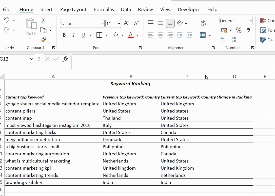
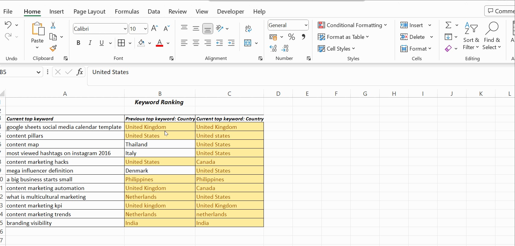
7.4 Example Scenario Using VLOOKUP

Column A contains a list of top keywords in a blog, and column B is the parent keyword. The resulting comparison must return all the ranking keywords in the blog.

The VLOOKUP() is applied in cell C4 as =VLOOKUP(A4, £B£4:£B£15,1,0).

Drag the cell to apply the formula in all the cells below C4. You will find the result in column C with the current and the matching parent keywords. The formula in Excel to compare two columns using VLOOKUP is as follows.

VLOOKUP(A4,..,..,..) – This takes the value in cell A4.

VLOOKUP(A4, £B£4:£B£15,..,..) – This compares all the values in cells from B4 to B15. That’s why the cells in range B4:B15 are locked using absolute reference. The £ symbol before the cell reference is called an absolute reference.

VLOOKUP(A4, £B£4:£B£15,1,..) – The third argument is the col_index_num, which mentions the position of the column to compare from the lookup value A4.

In the above example, the current top keyword is in column A, and the column with which it has to be compared is 1 column away. Hence, the value 1.

VLOOKUP(A4, £B£4:£B£15,1,0) – The last argument takes a logical value, either 0 or 1.

If you wish to find the exact match, mention 0(zero). If you want VLOOKUP() to return a closet match sorted in ascending order, mention 1 in this argument.

8. Comparing Multiple Columns

While the examples above focus on comparing two columns, Excel also allows you to compare multiple columns using a combination of formulas and functions.

8.1 Using IF and AND Functions

To compare three or more columns and find matches in all cells, you can use the IF() function with the AND() function.

Formula Syntax

=IF(AND(A2=B2, A2=C2), "Full Match", "")

This formula returns “Full Match” if the values in cells A2, B2, and C2 are all the same. Otherwise, it returns an empty string.

Example

Column A	Column B	Column C	Comparison Result
100	100	100	Full Match
100	100	101
101	101	101	Full Match

8.2 Using IF and OR Functions

To find matches in any two cells in the same row, you can use the IF() function with the OR() function.

Formula Syntax

=IF(OR(A2=B2, B2=C2, A2=C2), "Match", "")

This formula returns “Match” if any two of the values in cells A2, B2, and C2 are the same. Otherwise, it returns an empty string.

Example

Column A	Column B	Column C	Comparison Result
100	100	101	Match
100	101	102
101	101	102	Match

9. Advanced Techniques for Column Comparison

For more complex scenarios, you can use advanced techniques such as array formulas and custom functions to compare columns in Excel.

9.1 Array Formulas

Array formulas allow you to perform calculations on multiple values at once. This can be useful for comparing columns based on complex criteria.

Example

To compare two columns and return an array of TRUE/FALSE values indicating whether each row matches, you can use the following array formula:

=A1:A10=B1:B10

To enter this formula as an array formula, press Ctrl+Shift+Enter.

9.2 Custom Functions (VBA)

If you need to perform a specific type of column comparison that is not supported by built-in Excel functions, you can create a custom function using Visual Basic for Applications (VBA).

Example

To create a custom function that compares two columns and returns “Match” if the values are within a certain tolerance, you can use the following VBA code:

Function CompareWithTolerance(value1 As Double, value2 As Double, tolerance As Double) As String
    If Abs(value1 - value2) <= tolerance Then
        CompareWithTolerance = "Match"
    Else
        CompareWithTolerance = "Not Match"
    End If
End Function

You can then use this function in your Excel spreadsheet as follows:

=CompareWithTolerance(A1, B1, 0.1)

This formula compares the values in cells A1 and B1 and returns “Match” if they are within 0.1 of each other.

10. Troubleshooting Common Issues

When comparing columns in Excel, you may encounter some common issues. Here are some tips for troubleshooting these issues:

10.1 Incorrect Results

If you are getting incorrect results, double-check your formulas and ensure that you are using the correct functions and cell references.

10.2 Case Sensitivity

If you need to perform a case-sensitive comparison, use the EXACT function.

10.3 Formatting Differences

If you are comparing numbers or dates, ensure that the formatting is consistent across both columns.

10.4 Hidden Characters

Hidden characters, such as spaces or non-printing characters, can cause comparisons to fail. Use the TRIM function to remove leading and trailing spaces, and the CLEAN function to remove non-printing characters.

10.5 Error Values

If you encounter error values, such as #N/A or #VALUE!, troubleshoot the underlying cause of the error and ensure that your formulas are correctly referencing valid data.

Frequently Asked Questions

1. How do you compare two columns in Excel to find differences?

To compare two columns in Excel and find differences, you can use the IF function along with the equals operator (=). For example, the formula =IF(A1=B1, "Match", "Difference") will return “Match” if the values in cells A1 and B1 are the same, and “Difference” if they are different. Drag this formula down to apply it to all rows in the columns you are comparing.

2. How can I highlight differences between two columns in Excel?

You can highlight differences between two columns in Excel using conditional formatting. Select the columns you want to compare, then go to Home > Conditional Formatting > New Rule. Choose “Use a formula to determine which cells to format” and enter a formula like =A1<>B1. Set the desired formatting style (e.g., fill color) and click OK. This will highlight all cells where the values in the two columns are different.

3. How do I compare two columns for matching text?

To compare two columns for matching text, you can use the EXACT function. This function is case-sensitive and returns TRUE if the text in two cells is exactly the same, including capitalization. Use the formula =IF(EXACT(A1, B1), "Match", "Not Match") to compare the text in cells A1 and B1.

4. Can I compare two columns in different Excel sheets?

Yes, you can compare two columns in different Excel sheets. When writing your formula, reference the cells in the other sheet by including the sheet name followed by an exclamation mark (!). For example, to compare cell A1 in Sheet1 with cell A1 in Sheet2, use the formula =IF(Sheet1!A1=Sheet2!A1, "Match", "Not Match") in Sheet3.

5. How do I ignore case when comparing two columns in Excel?

To ignore case when comparing two columns in Excel, you can use the UPPER or LOWER functions to convert the text to the same case before comparing. For example, the formula =IF(UPPER(A1)=UPPER(B1), "Match", "Not Match") will compare the text in cells A1 and B1, ignoring case.

6. How can I compare two columns and extract the differences into a new column?

To compare two columns and extract the differences into a new column, you can use the IF function in combination with other functions like VLOOKUP or INDEX/MATCH. For example, if you want to find values in Column A that are not in Column B, you can use the formula =IF(ISERROR(VLOOKUP(A1,B:B,1,FALSE)),A1,""). This will return the value from Column A if it is not found in Column B, and an empty string if it is.

7. What is the best way to compare two large columns of data in Excel?

The best way to compare two large columns of data in Excel is to use a combination of conditional formatting and formulas. Use conditional formatting to quickly highlight differences or duplicates, and use formulas like IF, VLOOKUP, or COUNTIF to perform more complex comparisons and extract specific results. For very large datasets, consider using Power Query for more efficient data manipulation.

8. How do I find unique values in two columns in Excel?

To find unique values in two columns in Excel, you can use the COUNTIF function. First, combine the two columns into a single column. Then, in a new column, use the formula =IF(COUNTIF($A$1:$A$100,A1)=1,A1,"") to identify unique values. This formula counts the number of times each value appears in the combined column and returns the value if it appears only once.

9. How can I compare two columns and count the number of matches?

To compare two columns and count the number of matches, you can use the SUMPRODUCT function along with the equals operator (=). The formula =SUMPRODUCT(--(A1:A100=B1:B100)) will count the number of rows where the values in Column A and Column B are the same.

10. How do I compare two columns and identify missing values in one column compared to another?

To compare two columns and identify missing values in one column compared to another, you can use the VLOOKUP function. For example, if you want to find values in Column A that are not in Column B, use the formula =IF(ISERROR(VLOOKUP(A1,B:B,1,FALSE)),"Missing",""). This will return “Missing” if the value in Column A is not found in Column B.

Conclusion

Comparing two columns in Excel is a fundamental skill for data analysis, validation, and cleansing. Whether you use the equals operator, IF condition, EXACT function, conditional formatting, or lookup functions, Excel provides a variety of tools to streamline the comparison process. By mastering these techniques, you can ensure data integrity, identify inconsistencies, and make informed decisions based on accurate data.

Visit COMPARE.EDU.VN for more in-depth tutorials and resources to enhance your Excel skills and improve your data analysis capabilities.

Ready to make data-driven decisions with confidence? Explore the power of comparison at compare.edu.vn. Our comprehensive guides and tutorials will help you master Excel and other tools for effective data analysis. Visit us today at 333 Comparison Plaza, Choice City, CA 90210, United States, or contact us via Whatsapp at +1 (626) 555-9090. Start comparing and start succeeding.