**How to Compare Two Columns in Excel Using Formula?**

How To Compare Two Columns In Excel Using Formula is a common question for data analysts. Comparing two columns in Excel using formulas can greatly streamline your data analysis process, and at COMPARE.EDU.VN, we provide comprehensive guides to help you master these techniques. Learn effective methods for data validation, error detection, and data comparison. Explore techniques for data reconciliation and matching criteria.

1. Why Is Comparing Two Columns in Excel Useful?

Excel is a versatile tool for data storage, manipulation, and decision-making. While it excels at formatting text and organizing data, its ability to compare two columns is particularly useful for data analysts. By comparing columns across the same or different spreadsheets, analysts can make informed decisions based on accurate data insights. Manually comparing columns is time-consuming and prone to errors, but Excel’s comparison features provide a streamlined, efficient way to determine whether cells contain matching data. Excel can display results as TRUE/FALSE, Match/Not Match, or other user-defined messages, making the comparison process clear and customizable.

2. What Are the Methods to Compare Two Columns in Excel?

When you have data in two columns, tables, or spreadsheets, you may often need to compare them to see what data is missing or present in both. Comparisons can happen in many different ways for different reasons. Here’s a breakdown of methods to compare two columns:

Highlighting unique or duplicate values using functions.
Displaying unique or duplicate cells using conditional formatting or formulas.
Row-by-row comparison.
Using LOOKUP formulas.

3. How to Compare Two Columns in Excel with the Equals Operator

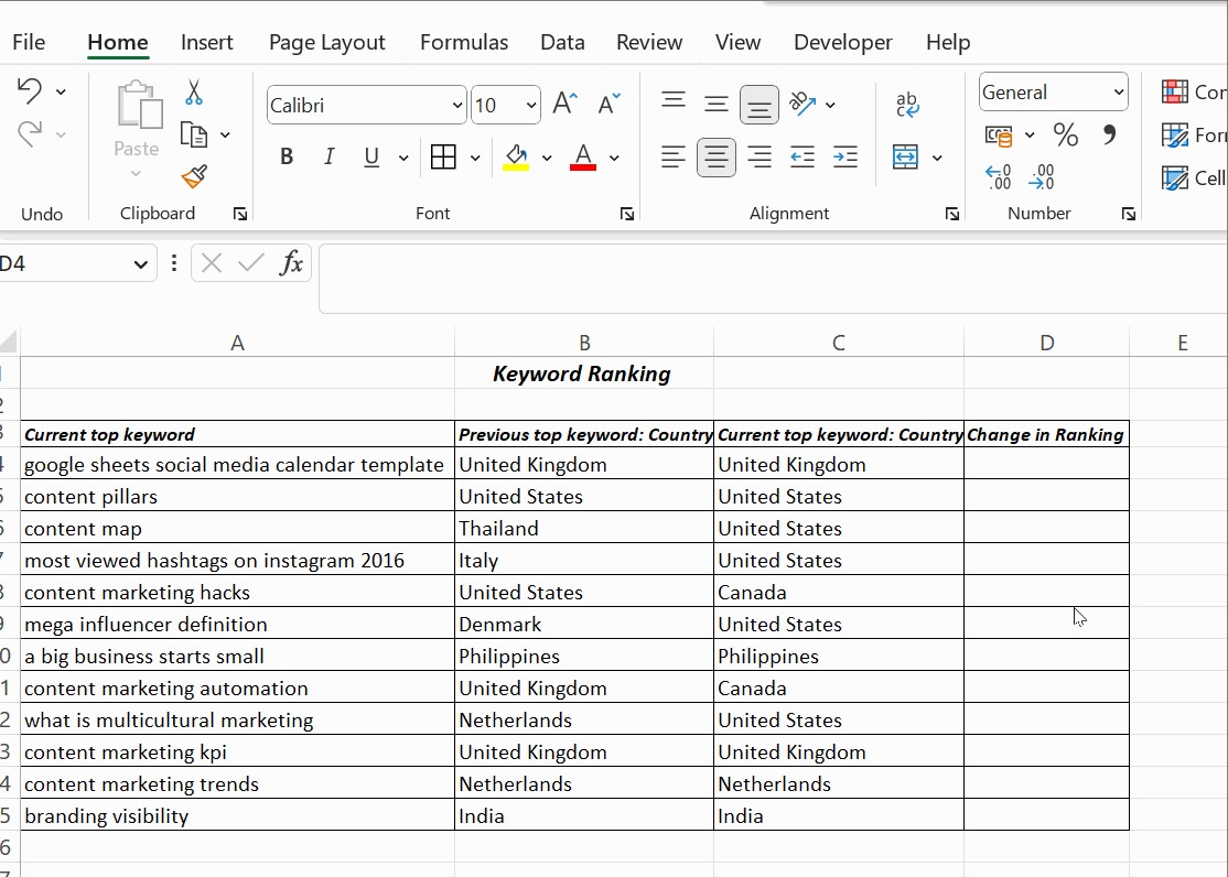
You can compare two columns, row by row, and find the matching data by returning the result as Match or Not Match. The formula used is =column1=column2, and by default, Excel returns a True if there’s a match or else False.

In cell D4, insert the formula =B4=C4 and press Enter. Then, drag it down to the end of the table. The formula returns TRUE if the values in compared columns are the same or returns FALSE if the values differ.

4. How to Compare Two Columns in Excel Using the IF Condition

You can compare two columns using the IF condition in Excel. The formula to compare two columns is =IF(B4=C4,”Yes”,” ”). It returns the result as Yes against the rows that contain matching values, and the remaining rows are left empty.

The same formula can identify and return the mismatching values. You need to include an additional argument, No, when the IF condition proves false. The formula is =IF(B4=C4,”Yes”,”No”).

To compare two columns in Excel for differences, replace the equals sign with the non-equality sign (<>). The formula is =IF(A2<>B2,”Match”,”Not a Match ”).

5. How to Compare Two Columns in Excel Using the EXACT() Function?

If you noticed in the previous screenshot, the formula returned a Yes for matching results that had different capitalizations. For instance, the country names had different capitalizations in rows 5, 13, and 14. The IF() returned Yes while comparing two columns containing Netherlands and netherlands, with n in lower case.

If you wish the capitalizations to be identical, use EXACT() when comparing two Excel columns and IF().

The EXACT() function compares two text strings and returns Yes only if they have the same capitalizations.

EXACT is case-sensitive but ignores formatting differences. The syntax is =EXACT(text1,text2). It takes two arguments, text1 and text2; both are required when using this function.

Let’s look at some examples. This time, EXACT() is used along with IF().

Use the formula =IF(EXACT(B4,C4), “Match”, “Mismatched”) for the IF condition to be case sensitive.

As you can observe, it returns the result as Mismatched for columns with matching results yet mismatched capitalizations.

The execution of the formula is as follows: first, the inner function is executed, and the result is returned. In the above example, the EXACT() function returns a false value to the outer function IF.

The general working of the IF condition is that if it returns true, the first argument in the function is returned. Or the second argument is returned as false.

6. How to Compare Two Columns in Excel Using Conditional Formatting?

Click Home, then on Styles.

Then, follow these steps Conditional Formatting → Highlight Cell Rules → Duplicate Values.

You get a dialogue box, as shown below. From there, you must choose the values from the drop-down menu.

Apply the formatting condition on the cells. You can choose any conditions; Duplicate or Unique.

Format cells that contain: (options) values with (options).

Use Conditional Formatting to find and highlight the data that are present in both columns. Before using conditional formatting, select the columns required for comparison.

Choose Duplicate if you wish to find the names in both columns. To highlight it, choose any options: filling with colour, changing the text colour, or changing the cell border.

The last option is a Custom Format. Choose this option if you wish to highlight the cell with a colour of your choice other than the ones specified in the drop-down menu.

Another option that you can use is ‘Unique.’ Use this option if you are interested in highlighting the cells that contain data that is not repeated. That is, you wish to highlight the unique cells.

Instead of selecting Duplicate, choose Unique from the drop-down list, and apply any options, such as filling with colour, changing the text colour, or changing the cell border.

Tip: If you wish to clear the formatting you performed on the cells, click Conditional Formatting → Clear Rules → Clear Rules from Selected Cells.

You can use conditional formatting when you don’t want a third column showing the results comparing the two columns. Highlighting duplicate (matching) and unique (different) data to show which rows have the same data.

Additionally, you can use an extra column to explicitly display values indicating whether the data matches, which works for smaller tables. Alternatively, you may need to use more complex methods for large spreadsheets.

7. How to Compare Two Columns in Excel Using Lookup Function

The LOOKUP function searches for a particular value in a row or column. It returns the corresponding value from another row or column. There are various lookup functions, viz, HLOOKUP, VLOOKUP, and XLOOKUP, where H and V stand for horizontal and vertical, and the XLOOKUP function is a combination of both LOOKUP and VLOOKUP.

The example below is to compare two columns in Excel for differences using VLOOKUP().

Column A contains a list of top keywords in a blog, and column B is the parent keyword. The resulting comparison must return all the ranking keywords in the blog.

The VLOOKUP() is applied in cell C4 as =VLOOKUP(A4, £B£4:£B£15,1,0).

Drag the cell to apply the formula in all the cells below C4. You will find the result in column C with the current and the matching parent keywords. The formula in Excel to compare two columns using VLOOKUP is as follows.

VLOOKUP(A4,..,..,..) – This takes the value in cell A4.
VLOOKUP(A4, £B£4:£B£15,..,..) – This compares all the values in cells from B4 to B15. That’s why the cells in range B4:B15 are locked using absolute reference. The £ symbol before the cell reference is called an absolute reference.
VLOOKUP(A4, £B£4:£B£15,1,..) – The third argument is the col_index_num, which mentions the position of the column to compare from the lookup value A4.

In the above example, the current top keyword is in column A, and the column with which it has to be compared is 1 column away. Hence, the value 1.

VLOOKUP(A4, £B£4:£B£15,1,0) – The last argument takes a logical value, either 0 or 1.

If you wish to find the exact match, mention 0(zero). If you want VLOOKUP() to return a closet match sorted in ascending order, mention 1 in this argument.

8. In-Depth Analysis of Using Formulas for Column Comparison

Using formulas to compare two columns in Excel provides flexibility and precision. Here’s an in-depth look at various formulas and their applications:

8.1. Using the EXACT Function

The EXACT function ensures case-sensitive comparisons, which is vital when distinguishing between entries like “Apple” and “apple”.

Syntax: =EXACT(text1, text2)
Application: =IF(EXACT(A1, B1), "Match", "No Match")

8.2. Combining IF and ISNA with VLOOKUP

This combination identifies values in one column that are not present in another.

Syntax: =IF(ISNA(VLOOKUP(value, table, col_index, [range_lookup])), "Not Found", "Found")
Application: =IF(ISNA(VLOOKUP(A1, $B$1:$B$10, 1, FALSE)), "Missing in Column B", "Present in Column B")

8.3. Using COUNTIF for Identifying Duplicates

COUNTIF helps find duplicates across two columns by counting how many times a value from one column appears in another.

Syntax: =COUNTIF(range, criteria)
Application: =IF(COUNTIF($B$1:$B$10, A1)>0, "Duplicate", "Unique")

8.4. Implementing Array Formulas

Array formulas can perform multiple calculations in one go, making them efficient for complex comparisons.

Syntax: {=SUM(IF(A1:A10=B1:B10, 1, 0))} (Note: Enter as an array formula using Ctrl+Shift+Enter)
Application: This formula counts the number of rows where the values in column A match those in column B.

8.5. Employing the XOR Logic

The XOR (exclusive OR) logic identifies rows where values in two columns are different.

Syntax: =IF(A1<>B1, "Different", "Same")
Application: This flags any differences between corresponding rows in columns A and B.

8.6. Advanced Conditional Formatting with Formulas

Beyond basic duplicate highlighting, conditional formatting can be combined with formulas for more complex comparisons.

Custom Rule Formula: =A1=B1
Application: This highlights matching cells across columns, providing a visual comparison.

8.7. Comparing Columns with Multiple Criteria

When comparisons depend on multiple conditions, use AND or OR functions within your formulas.

Syntax: =IF(AND(condition1, condition2), "Match", "No Match")
Application: =IF(AND(A1>10, B1<20), "Meets Both Criteria", "Does Not Meet Both")

By mastering these formulas, users can perform detailed and precise comparisons, tailored to their specific data analysis needs. Each technique offers unique benefits, from case-sensitive matching to identifying duplicates and differences, providing a comprehensive toolkit for Excel users.

9. Step-by-Step Guide to Comparing Two Columns Using a Formula

To effectively compare two columns in Excel using a formula, follow these detailed steps. This guide assumes you want to identify matching entries between two columns, A and B, and display the result in column C.

9.1. Open Your Excel Worksheet

Start by opening the Excel worksheet that contains the two columns you wish to compare. Ensure that the data is properly organized and ready for comparison.

9.2. Select the First Cell in the Result Column

In this example, we will use column C to display the results. Select the first cell in column C, which corresponds to the first row of data in columns A and B (e.g., cell C1).

9.3. Enter the Comparison Formula

In cell C1, enter the formula to compare the values in cells A1 and B1. Here are a few options:

Basic Match Check:
- Enter the formula: =IF(A1=B1, "Match", "No Match")
- This formula checks if the value in cell A1 is equal to the value in cell B1. If they are equal, it displays “Match”; otherwise, it displays “No Match”.
Case-Sensitive Match Check:
- Enter the formula: =IF(EXACT(A1, B1), "Match", "No Match")
- This formula uses the EXACT function to perform a case-sensitive comparison. It ensures that the values in A1 and B1 are exactly the same, including capitalization.
Check for Differences:
- Enter the formula: =IF(A1<>B1, "Different", "Same")
- This formula checks if the value in cell A1 is different from the value in cell B1. If they are different, it displays “Different”; otherwise, it displays “Same”.

9.4. Apply the Formula to the Rest of the Column

After entering the formula in cell C1, you need to apply it to the rest of the cells in column C to compare all corresponding rows in columns A and B.

Select Cell C1: Click on cell C1 where you entered the formula.
Locate the Fill Handle: Move your cursor to the bottom-right corner of cell C1. You will see a small square, known as the fill handle.
Drag the Fill Handle: Click and drag the fill handle down to the last row of your data in columns A and B. Excel will automatically apply the formula to all the cells you drag over, adjusting the cell references accordingly.
Alternatively, Double-Click the Fill Handle: Instead of dragging, you can double-click the fill handle. Excel will automatically fill the formula down to the last row that contains data in the adjacent columns (A and B).

9.5. Review the Results

Column C will now display the comparison results for each row. You can quickly scan the column to identify matches, differences, or any other criteria you defined in your formula.

9.6. Customize the Output (Optional)

You can customize the output of the formula to display different text or values based on your specific needs. For example:

Instead of “Match” and “No Match”, you can use “Yes” and “No”, or any other relevant terms.
You can also use numbers (e.g., 1 for “Match”, 0 for “No Match”) if you need to perform further calculations based on the comparison results.

9.7. Use Conditional Formatting for Visual Highlighting (Optional)

To make the comparison results even more visually clear, you can use conditional formatting to highlight the matching or non-matching cells.

Select Column C: Click on the column header (C) to select the entire column of results.
Go to Conditional Formatting: Click on “Conditional Formatting” in the “Home” tab.
Choose Highlighting Rules: Select “Highlight Cells Rules” and choose the appropriate rule:
- Equals To: Use this to highlight cells that contain a specific text value (e.g., “Match” or “No Match”).
- Text that Contains: Use this to highlight cells that contain a specific word or phrase.
Set the Formatting: Choose the formatting style you want to apply (e.g., fill color, text color) and click “OK”.

9.8. Example Scenario

Suppose you have two columns with customer names (Column A) and a list of registered users (Column B). You want to identify which customers are also registered users.

Enter the Formula: In cell C1, enter =IF(ISNA(VLOOKUP(A1, $B$1:$B$100, 1, FALSE)), "Not Registered", "Registered"). This formula checks if the customer name in A1 is found in the list of registered users in B1:B100.
Apply the Formula: Drag the fill handle down to apply the formula to all customer names in Column A.
Review the Results: Column C will now show “Registered” or “Not Registered” for each customer, indicating whether they are in the registered users list.

10. FAQ: How to Compare Two Columns in Excel Using Formulas?

10.1. How do you compare two columns in Excel?

When comparing two columns in Excel, one method is to select both columns of data, select Home → Find & Select → Go To Special → Row Differences, and click OK. The matching data cells across the columns’ rows are white, and unmatched cells appear in gray.

10.2. How to compare three or more columns in Excel?

To find matches in all cells when the table has three or more columns, use an IF() with AND statement. The formula is =IF(AND(A2=B2, A2=C2), “Full match”, “”).

The formula to find matches in any two cells in the same row is =IF(OR(A2=B2, B2=C2, A2=C2), “Match”, “”).

10.3. Can I compare two columns for differences in Excel?

Yes, you can compare two columns for differences in Excel using the IF function along with the not equal to operator (<>). For example, the formula =IF(A1<>B1, "Different", "Same") will return “Different” if the values in cells A1 and B1 are not the same, and “Same” if they are identical. This allows you to quickly identify discrepancies between the two columns.

10.4. How can I perform a case-sensitive comparison in Excel?

To perform a case-sensitive comparison in Excel, you can use the EXACT function. The EXACT function checks if two text strings are identical, including their capitalization. For example, the formula =IF(EXACT(A1, B1), "Match", "No Match") will return “Match” only if the values in cells A1 and B1 are exactly the same, including capitalization. If the capitalization differs, it will return “No Match”.

10.5. Is there a way to highlight differences between two columns automatically?

Yes, you can automatically highlight differences between two columns using conditional formatting with a formula. Here’s how:

Select the Range: Select the range of cells you want to compare (e.g., columns A and B).
Open Conditional Formatting: Go to the “Home” tab, click on “Conditional Formatting,” and select “New Rule.”
Use a Formula: Choose “Use a formula to determine which cells to format.”
Enter the Formula: Enter a formula that checks for differences, such as =A1<>B1.
Set the Formatting: Click on “Format,” choose the desired formatting style (e.g., fill color, text color), and click “OK.”
Apply the Rule: Click “OK” to apply the conditional formatting rule.

Excel will now automatically highlight any cells where the values in columns A and B differ.

10.6. How do I find values in one column that are not in another?

To find values in one column that are not present in another, you can use a combination of the VLOOKUP and ISNA functions. Here’s how:

Enter the Formula: In an empty column (e.g., column C), enter the formula =IF(ISNA(VLOOKUP(A1, $B$1:$B$100, 1, FALSE)), "Not Found", "Found").
- A1 is the first cell in the column you want to check (e.g., column A).
- $B$1:$B$100 is the range of cells in the other column (e.g., column B). Adjust the range as needed.
- FALSE ensures an exact match.
Apply the Formula: Drag the fill handle down to apply the formula to all cells in column A.

Column C will now show “Not Found” for values in column A that are not present in column B, and “Found” for values that are present.

10.7. Can I compare two columns and return a value from a third column if there’s a match?

Yes, you can compare two columns and return a value from a third column if there’s a match using the IF and VLOOKUP functions. Here’s the formula:

=IF(NOT(ISNA(VLOOKUP(A1, $B$1:$C$100, 2, FALSE))), VLOOKUP(A1, $B$1:$C$100, 2, FALSE), "")

A1 is the cell in the first column you want to check.
$B$1:$C$100 is the range containing the second column to compare (B) and the third column from which to return the value (C).
The formula checks if the value in A1 is found in column B. If it is, it returns the corresponding value from column C; otherwise, it returns an empty string.

10.8. How do I compare two columns and count the number of matches?

To compare two columns and count the number of matches, you can use the SUMPRODUCT function along with a comparison. Here’s the formula:

=SUMPRODUCT(--(A1:A100=B1:B100))

A1:A100 and B1:B100 are the ranges of cells you want to compare.
The formula compares each cell in column A with the corresponding cell in column B and counts the number of matches.

10.9. Is it possible to ignore case when comparing two columns?

Yes, it is possible to ignore case when comparing two columns by using the UPPER or LOWER functions. Here’s how:

Using UPPER:
- Enter the formula: =IF(UPPER(A1)=UPPER(B1), "Match", "No Match")
- This formula converts the values in both cells to uppercase before comparing them, effectively ignoring case.
Using LOWER:
- Enter the formula: =IF(LOWER(A1)=LOWER(B1), "Match", "No Match")
- This formula converts the values in both cells to lowercase before comparing them, also ignoring case.

10.10. How can I compare two columns and return “Match” only if multiple criteria are met?

You can compare two columns and return “Match” only if multiple criteria are met by using the AND function within an IF statement. Here’s how:

=IF(AND(A1=B1, C1=D1, E1=F1), "Match", "No Match")

This formula checks if the values in cells A1 and B1, C1 and D1, and E1 and F1 are all equal. If all conditions are true, it returns “Match”; otherwise, it returns “No Match”. Adjust the cell references and conditions as needed to fit your specific criteria.

Conclusion

Comparing two columns in Excel can be straightforward when the table is small. However, when dealing with vast spreadsheets or multiple linked spreadsheets, the comparison process becomes more complex. This tutorial provided a detailed overview of how to compare two columns in Excel, showcasing various options to match data in single columns, multiple columns, and multiple spreadsheets.

For further assistance and to explore more in-depth guides, visit COMPARE.EDU.VN. Our resources are designed to help you make informed decisions and streamline your data analysis tasks. Contact us at 333 Comparison Plaza, Choice City, CA 90210, United States or via WhatsApp at +1 (626) 555-9090.

By using COMPARE.EDU.VN, you gain access to comprehensive comparisons that help you make informed decisions efficiently. Don’t let the complexity of data analysis slow you down. Visit compare.edu.vn today and discover how easy it can be to compare, contrast, and choose the best options for your needs using lookup functions, data validation techniques, and matching datasets efficiently.

How to Compare Two Columns in Excel Using Formula?