Comparing two columns in Excel for identical values can be achieved efficiently using various built-in features and formulas, ensuring data accuracy and streamlining your workflow. At COMPARE.EDU.VN, we provide comprehensive guides to help you master these techniques. By understanding these methods, you can quickly identify matches and discrepancies, enhancing your data analysis capabilities and saving valuable time. Explore different approaches such as conditional formatting, the equals operator, and the VLOOKUP function to find the best fit for your needs.
1. What Does Comparing Columns in Excel Mean?
Comparing columns in Excel refers to the process of checking corresponding cells in two or more columns to identify similarities, differences, or matches. This can be useful for tasks like data validation, finding duplicates, or updating records. By comparing data between columns, you can ensure data integrity and make informed decisions. Excel’s built-in tools and functions like conditional formatting, the equals operator, VLOOKUP, and IF formulas make this process efficient.
2. How To Compare Two Columns In Excel Effectively
Here are several effective methods to compare two columns in Excel:
- Conditional Formatting in Excel
- Using the Equals Operator
- Using VLOOKUP Function
- Using the IF Formula
- Using the EXACT Formula
Let’s explore each method in detail.
2.1. Conditional Formatting in Excel
Conditional Formatting in Excel is one of the simplest ways to compare columns. It allows you to highlight duplicate or unique values quickly, making it easy to spot matches or discrepancies.
Step 1: Select All Cells in the Spreadsheet
First, select all the cells in the spreadsheet that you want to compare. This ensures that the conditional formatting will be applied across the entire dataset.
Step 2: Navigate to Conditional Formatting
Go to the “Home” tab on the Excel ribbon. In the “Styles” group, click on “Conditional Formatting.” A dropdown menu will appear with various options.
Step 3: Select “Highlight Cells Rules”
From the dropdown menu, select “Highlight Cells Rules.” Another submenu will appear. Choose either “Duplicate Values” or “Unique Values” depending on what you are looking for.
A. Duplicate Values
Choosing “Duplicate Values” will highlight all cells that appear more than once within the selected range. This is useful for identifying matching data across the columns.
- Select the Range: Select the two columns you want to compare.
- Apply Conditional Formatting: Go to Home > Conditional Formatting > Highlight Cells Rules > Duplicate Values.
- Choose Formatting: Select the formatting style (e.g., fill color) and click OK.
B. Unique Values
Selecting “Unique Values” will highlight all cells that appear only once within the selected range. This is helpful for finding discrepancies or unique entries in your data.
- Select the Range: Select the two columns you want to compare.
- Apply Conditional Formatting: Go to Home > Conditional Formatting > Highlight Cells Rules > Unique Values.
- Choose Formatting: Select the formatting style and click OK.
2.2. Using the Equals Operator
Another straightforward way to compare columns in Excel is by using the equals operator (=). This method involves creating a new column that displays TRUE or FALSE based on whether the values in the corresponding rows of the two columns match.
Step 1: Create a New Result Column
Insert a new column next to the columns you want to compare. This column will display the results of the comparison.
Step 2: Add the Formula for Individual Cell Comparison
In the first cell of the new column, enter the formula =A2=B2 (assuming your data starts in row 2). This formula compares the value in cell A2 with the value in cell B2.
Step 3: Apply the Formula to All Cells
Drag the fill handle (the small square at the bottom-right of the cell) down to apply the formula to all the rows you want to compare.
Step 4: Interpret the Results
Excel will display TRUE for every successful comparison (i.e., when the values in both cells are the same) and FALSE for every unsuccessful comparison (i.e., when the values differ).
Step 5: Customize Messages Using the IF Clause (Optional)
You can make the results more user-friendly by using the IF clause to display custom messages instead of TRUE and FALSE. For example, the formula =IF(A2=B2, "Match", "No Match") will display “Match” if the values are the same and “No Match” if they are different.
2.3. Using VLOOKUP Function
The VLOOKUP function is useful for comparing two columns in Excel when you want to check if values from one column exist in another column. It searches for a value in the first column of a range and returns a corresponding value from another column in the same range.
Syntax:
=VLOOKUP(lookup_value, table_array, col_index_num, [range_lookup])
- lookup_value: The value you want to search for.
- table_array: The range in which to search.
- col_index_num: The column number in the range from which to return a value.
- range_lookup: An optional argument. Use FALSE for an exact match.
Step 1: Create a New Result Column
Insert a new column where the results of the VLOOKUP function will be displayed.
Step 2: Add the VLOOKUP Formula to Compare Individual Cells
In the first cell of the new column, enter the VLOOKUP formula. For example, if you want to check if the values in column A exist in column B, you can use the following formula:
=VLOOKUP(A2, B:B, 1, FALSE)
This formula searches for the value in cell A2 within column B. The 1 indicates that it should return the value from the first column of the range (which is column B in this case), and FALSE ensures an exact match.
Step 3: Drag the Formula to All the Cells
Drag the fill handle down to apply the formula to all the rows you want to compare.
Step 4: Interpret the Results
If the value from column A is found in column B, the VLOOKUP function will return that value. If the value is not found, it will return a #N/A error.
Step 5: Handle Errors Using the IFERROR Clause (Optional)
To avoid displaying #N/A errors, you can modify the formula using the IFERROR clause. This allows you to display a custom message when a value is not found. For example:
=IFERROR(VLOOKUP(A2, B:B, 1, FALSE), "Not Found")
This formula will display “Not Found” instead of #N/A when the value from column A is not found in column B.
Step 6: Adjust for Real-World Scenarios (Optional)
In real-world scenarios, you might encounter slight variations in the data that can cause the VLOOKUP function to return incorrect results. For example, if one cell contains “Ford India” and another contains “Ford,” the standard VLOOKUP might return “Not Found” even though the values are similar.
To address this, you can use wildcards in the lookup value. For example:
=IFERROR(VLOOKUP(A2&"*", B:B, 1, FALSE), "Not Found")
The &"*" adds a wildcard to the lookup value, which allows VLOOKUP to find the value even if it is not an exact match.
2.4. Compare 2 Columns Using the IF Formula
The IF formula is a versatile tool for comparing two columns in Excel. It allows you to display a specific result if the values in the corresponding rows match and a different result if they don’t.
Syntax:
IF Formula: =IF(A2=B2, “Match”, ” “)
This formula checks if the value in cell A2 is equal to the value in cell B2. If it is, the formula returns “Match.” If it isn’t, the formula returns a blank space.
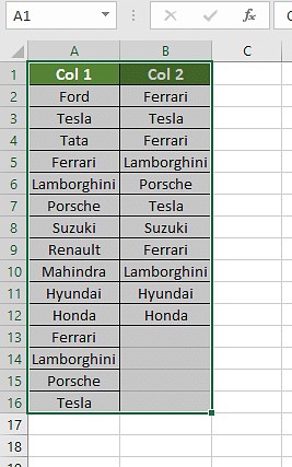
Step 1: Set Up Your Data
Ensure you have two columns of data that you want to compare. For this example, let’s assume your data is in columns A and B, starting from row 2.
Step 2: Enter the IF Formula
In the first cell of the result column (e.g., column C, row 2), enter the IF formula. For example:
=IF(A2=B2, "Same car brands", "Different car brands")
This formula will display “Same car brands” if the values in A2 and B2 are the same and “Different car brands” if they are different.
Step 3: Drag the Formula Down
Drag the fill handle (the small square at the bottom-right of the cell) down to apply the formula to all the rows you want to compare.
2.5. Compare Using the EXACT Formula
The EXACT formula is used to compare two strings in Excel. It is case-sensitive, meaning it distinguishes between uppercase and lowercase letters. This makes it useful when you need to ensure that the values in two columns are exactly the same, including capitalization.
Syntax:
“=EXACT(A2, B2)”
This formula compares the value in cell A2 with the value in cell B2. If the values are exactly the same, including case, the formula returns TRUE. If they are not, the formula returns FALSE.
Step 1: Set Up Your Data
Ensure you have two columns of data that you want to compare. For this example, assume your data is in columns A and B, starting from row 2.
Step 2: Enter the EXACT Formula
In the first cell of the result column (e.g., column C, row 2), enter the EXACT formula. For example:
=EXACT(A2, B2)
This formula will return TRUE if the values in A2 and B2 are exactly the same (including case) and FALSE if they are not.
Step 3: Drag the Formula Down
Drag the fill handle (the small square at the bottom-right of the cell) down to apply the formula to all the rows you want to compare.
3. Which Comparison Method to Use in Each Scenario
3.1. Scenario 1: Comparing Two Columns in Excel Row-by-Row
To compare two columns in Excel row-by-row, use the following formulas:
=IF(A2 = B2, "match", " ")=IF(A2<>B2, "no match", " ")=IF(A2 = B2, "match", "no match")
If you need the results to be case-sensitive, then use the following formulas:
=IF(EXACT(A2, B2), "Match", " ")=IF(EXACT(A2, B2), "Match," "No match")
3.2. Scenario 2: Comparing Multiple Columns for Row Matches
If you need to compare and find the differences and similarities between more than two columns, then use the following formulas:
=IF(AND(A2=B2, A2=C2), "Complete match", " ")=IF(COUNTIF($A2:$E2, $A2)=4, "Complete match," "), where 4 is the number of columns you are comparing
If you want to compare columns with any two or more cells with the same values in the same row, then you might use the following formulas:
=IF(OR(A2=B2, B2=C2, A2=C2), "Match", "")=IF(COUNTIF(B2:D2,A2)+COUNTIF(C2:D2,B2)+(C2=D2)=0,"Unique","Match")
3.3. Scenario 3: Compare Two Columns for Matches and Differences
To compare two datasets, to find the unique values present in column A and not in column B one can use any of the formulas for finding the match and differences:
=IF(COUNTIF($B:$B, $A2)=0, "Not present in B", "")=IF(ISERROR(MATCH($A2,$B$2:$B$10,0)),"No present in B","")
You can use a single formula to get the result for matches and unique values:
=IF(COUNTIF($B:$B, $A2)=0, "No Present in B", "Present in B")
3.4. Scenario 4: Compare Two Lists and Pull Matching Data
To compare two lists and find the matching data, you can use the VLOOKUP function. You can also use the INDEX MATCH formula. You can use the following formulas for this scenario:
=VLOOKUP(D2, $A$2:$B$6, 2, FALSE)=INDEX($B$2:$B$6, MATCH($D2, $A$2:$A$6, 0))=XLOOKUP(D2, $A$2:$A$6, $B$2:$B$6)
A2, B2 and D2 are the first cells of three columns. 2 is the number of columns compared.
3.5. Scenario 5: Highlight Row Matches and Differences
You can create a conditional formatting formula that can highlight the rows that include identical values in all the columns. You can use the following formula for the desired result:
=AND($A2=$B2, $A2=$C2)
or
=COUNTIF($A2:$C2, $A2)=3
3 is the number of columns and A2, B2 and C2 are the top-most cells, to compare.
You can also use the following steps to find and highlight the matches and differences in Excel:
- Select the columns with the dataset you want to compare.
- Go to the editing group section on the Home tab, click the “Find and Select” drop-down, and choose “Go To Special.” Select Row Differences and click OK.
- The cells having different values than the cells compared in each row will be colored. To change the color click the Fill Color icon on and choose the color of your choice.
4. Streamline Your Data Analysis with COMPARE.EDU.VN
Comparing columns in Excel is essential for ensuring data accuracy and consistency. By mastering the techniques discussed, you can efficiently manage and analyze your data, making informed decisions with confidence.
At COMPARE.EDU.VN, we understand the challenges in comparing various options to make informed decisions. That’s why we provide comprehensive and objective comparisons across different products, services, and ideas.
Whether you’re a student comparing courses, a consumer evaluating products, or a professional analyzing solutions, COMPARE.EDU.VN offers the insights you need. Our detailed comparisons highlight the pros and cons, features, specifications, and user reviews, empowering you to choose the best option for your needs and budget.
Visit COMPARE.EDU.VN today to explore detailed comparisons and make smarter, more informed decisions. Let us help you simplify the comparison process and find the perfect fit for your unique requirements.
Contact Us:
- Address: 333 Comparison Plaza, Choice City, CA 90210, United States
- WhatsApp: +1 (626) 555-9090
- Website: compare.edu.vn
5. FAQs
5.1. How To Compare Two Columns in Excel?
One popular method for comparing two columns in Excel is to follow these steps: select both columns of data → go to the Home tab → click on Find & Select → choose Go To Special → select Row Differences → click OK.
5.2. Is It Possible To Compare Two Columns in Excel Using the Index-Match Function?
Yes, you can compare two columns in Excel using the Index-Match function by creating the required formula for the data required.
5.3. How To Compare Multiple Columns in Excel?
To compare multiple columns in Excel, you can use the conditional formatting option on the Home and format the setting to “duplicates” or “uniques”, and choose the desired color to highlight the values to compare multiple columns.
5.4. How Do You Compare Two Lists in Excel for Matches?
You can compare two lists in Excel using IF function, MATCH function or highlighting row differences.
5.5. How Can I Compare Columns and Highlight the First Occurrence of a Mismatch?
Use Conditional Formatting with a formula like =A1B1 to highlight cells where the values differ.
5.6. How Do I Compare Columns for Duplicates Only?
Use the formula =COUNTIF(B:B, A1)>0 to find duplicates between columns A and B.
5.7. Can I Compare Columns and Count the Number of Matches or Differences?
Yes, use formulas like =SUMPRODUCT(–(A1:A10=B1:B10)) to count matches or =COUNTIF(A1:A10, “B1:B10”) for differences.