**How Do I Compare Two Columns In Excel For Matching Values?**

How To Compare Two Columns In Excel For Matching Values? This process involves checking cells across columns to identify matches, a task made easy with tools like conditional formatting and VLOOKUP, as explored on COMPARE.EDU.VN. By understanding how to compare values, users can efficiently manage data discrepancies and ensure data accuracy. For advanced data analysis and insights, consider leveraging techniques like data validation and formula auditing.

1. What Does Comparing Columns in Excel Mean?

Comparing columns in Excel involves examining corresponding cells across different columns to determine if their values match or differ. This process is crucial for data validation, identifying duplicates, and ensuring data integrity. You can find detailed guides and comparison tools at COMPARE.EDU.VN.

2. What Are The Methods to Compare Two Columns in Excel?

Here are several effective methods to compare two columns in Excel:

1. Conditional Formatting
2. Equals Operator
3. VLOOKUP Function
4. IF Formula
5. EXACT Formula

Let’s dive into each method to understand how they work and when to use them effectively.

2.1. How to Use Conditional Formatting in Excel to Compare Columns

Conditional formatting in Excel is a simple and visual way to compare columns. It allows you to highlight duplicate or unique values, making it easy to spot differences or matches at a glance.

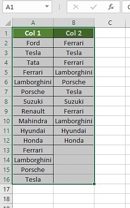
Step 1: Select Your Data

Start by selecting the columns you want to compare. Click and drag your cursor over the columns to highlight them.

Step 2: Access Conditional Formatting

Go to the “Home” tab on the Excel ribbon. In the “Styles” group, click on “Conditional Formatting.”

Step 3: Highlight Duplicate or Unique Values

A dropdown menu will appear. Select “Highlight Cells Rules,” and then choose either “Duplicate Values” or “Unique Values,” depending on what you’re looking for.

A. Highlighting Duplicate Values

Choosing “Duplicate Values” will highlight all cells that appear in both columns. This is useful for identifying common entries in your datasets.

B. Highlighting Unique Values

Selecting “Unique Values” will highlight cells that appear only in one of the selected columns. This is great for finding discrepancies or unique entries.

Step 4: Choose Your Formatting

A dialog box will open, allowing you to select the formatting style for the highlighted cells. You can choose from predefined styles or customize the fill color, text color, and more.

2.2. How to Use Equals Operator to Compare Columns in Excel

Using the equals operator (=) is a straightforward way to compare corresponding cells in two columns. This method returns TRUE if the values match and FALSE if they don’t.

Step 1: Create a Result Column

Insert a new column next to the columns you want to compare. This column will display the results of the comparison.

Step 2: Enter the Formula

In the first cell of the result column, enter the formula =A2=B2, where A2 and B2 are the first cells in the columns you’re comparing.

Step 3: Apply the Formula to the Entire Column

Drag the fill handle (the small square at the bottom-right of the cell) down to apply the formula to all the rows you want to compare.

Step 4: Customize the Result with an IF Clause (Optional)

To display custom messages instead of TRUE and FALSE, you can use the IF function. For example, the formula =IF(A2=B2, "Match", "No Match") will display “Match” if the values in A2 and B2 are the same, and “No Match” if they are different.

2.3. How to Use the VLOOKUP Function to Compare Columns in Excel

The VLOOKUP function is useful for finding matches between two columns and returning a corresponding value from another column. To compare two columns in Excel using VLOOKUP, follow these steps:

Step 1: Understand the VLOOKUP Syntax

The syntax for the VLOOKUP function is:

=VLOOKUP(lookup_value, table_array, col_index_num, [range_lookup])

• lookup_value: The value you want to find in the first column of the table.
• table_array: The range of cells that contains the table where you want to look for the value.
• col_index_num: The column number in the table_array from which to return a value.
• range_lookup: A logical value (TRUE or FALSE) that specifies whether you want an approximate or exact match. Use FALSE for an exact match.

Step 2: Set Up Your Data

Ensure that the column you want to look up values in (the “lookup column”) is to the left of the column containing the values you want to compare.

Step 3: Enter the VLOOKUP Formula

In the first cell of your result column, enter the VLOOKUP formula. For example, if you want to see if the values in column A exist in column C, and return a value from column D if there is a match, you can use the following formula in cell B2:

=VLOOKUP(A2, $C$2:$D$10, 2, FALSE)

In this formula:

• A2 is the lookup value (the value from column A that you want to find in column C).
• $C$2:$D$10 is the table array (the range of cells in columns C and D where you want to look for the value). The dollar signs make the reference absolute, so it doesn’t change when you drag the formula down.
• 2 is the column index number (the column in the table array from which to return a value). In this case, it’s column D.
• FALSE specifies that you want an exact match.

Step 4: Apply the Formula to the Entire Column

Drag the fill handle (the small square at the bottom-right of the cell) down to apply the formula to all the rows you want to compare.

Step 5: Handle Errors with IFERROR (Optional)

If a value in column A does not exist in column C, the VLOOKUP function will return an error (#N/A). To display a custom message instead of the error, you can use the IFERROR function. For example:

=IFERROR(VLOOKUP(A2, $C$2:$D$10, 2, FALSE), "Not Found")

This formula will display “Not Found” if the value in A2 is not found in column C.

Step 6: Adjust for Variations (Optional)

In some cases, the values in the columns you’re comparing may not be exactly the same. For example, one column might contain “Ford India,” while the other contains “Ford.” In these cases, you can use wildcards to broaden the search. For example:

=VLOOKUP(A2&"*", $C$2:$D$10, 2, FALSE)

The &"*" adds a wildcard to the lookup value, allowing it to match values that start with the same text but have additional characters.

2.4. How to Use the IF Formula to Compare Columns in Excel

The IF formula in Excel allows you to perform logical comparisons between two columns and display a specified result based on whether the comparison is true or false. This is particularly useful when you want to categorize the similarities or differences between values in two columns.

Step 1: Understand the IF Formula Syntax

The basic syntax for the IF formula is:

=IF(logical_test, value_if_true, value_if_false)

• logical_test: This is the condition you want to test. In this case, it will be a comparison between two cells in different columns.
• value_if_true: The value that the formula will return if the logical_test is true.
• value_if_false: The value that the formula will return if the logical_test is false.

Step 2: Set Up Your Data

Ensure you have the two columns you want to compare next to each other in your Excel sheet. For this example, we’ll assume you have data in columns A and B.

Step 3: Enter the IF Formula

In the first cell of your result column (e.g., column C), enter the IF formula to compare the corresponding cells in columns A and B. For example, if you want to check if the values in cell A2 are equal to the values in cell B2, you can use the following formula in cell C2:

=IF(A2=B2, "Match", "Different")

In this formula:

• A2=B2 is the logical test that checks if the values in cell A2 and cell B2 are equal.
• "Match" is the value that the formula will return if the values in A2 and B2 are the same.
• "Different" is the value that the formula will return if the values in A2 and B2 are different.

Step 4: Apply the Formula to the Entire Column

Drag the fill handle (the small square at the bottom-right of the cell) down to apply the formula to all the rows you want to compare. This will automatically adjust the cell references in the formula for each row.

2.5. How to Compare Columns Using the EXACT Formula in Excel

The EXACT formula in Excel is used to compare two strings and returns TRUE if they are exactly the same, including case. This formula is case-sensitive, meaning it distinguishes between uppercase and lowercase letters.

Step 1: Understand the EXACT Formula Syntax

The syntax for the EXACT formula is:

=EXACT(text1, text2)

• text1: The first text string you want to compare.
• text2: The second text string you want to compare.

Step 2: Set Up Your Data

Ensure that the two columns you want to compare are next to each other in your Excel sheet. For this example, we’ll assume you have data in columns A and B.

Step 3: Enter the EXACT Formula

In the first cell of your result column (e.g., column C), enter the EXACT formula to compare the corresponding cells in columns A and B. For example, if you want to check if the values in cell A2 are exactly the same as the values in cell B2, you can use the following formula in cell C2:

=EXACT(A2, B2)

In this formula:

• A2 is the first text string you want to compare (the value in cell A2).
• B2 is the second text string you want to compare (the value in cell B2).

Step 4: Apply the Formula to the Entire Column

Drag the fill handle (the small square at the bottom-right of the cell) down to apply the formula to all the rows you want to compare. This will automatically adjust the cell references in the formula for each row.

3. Which Comparison Method to Use in Each Scenario?

Choosing the right comparison method in Excel depends on your specific needs and the nature of your data. Here’s a guide to help you select the most appropriate method for various scenarios:

3.1. How to Compare Two Columns in Excel Row-by-Row?

When you need to compare two columns in Excel on a row-by-row basis, several formulas can help you identify matches and differences. Here are a few options, along with examples:

Basic Match and No Match:

• To display “Match” if the values in two cells are the same and a blank space if they are different, use the following formula:

  =IF(A2 = B2, "Match", " ")

• To display “No Match” if the values in two cells are different and a blank space if they are the same, use this formula:

  =IF(A2<>B2, "No Match", " ")

• For a more comprehensive result, you can display “Match” if the values are the same and “No Match” if they are different using the following formula:

  =IF(A2 = B2, "Match", "No Match")

Case-Sensitive Comparison:

If you need to perform a case-sensitive comparison, meaning that the formula should distinguish between uppercase and lowercase letters, you can use the EXACT function.

• To display “Match” only if the values are exactly the same (including case) and a blank space if they are different, use the following formula:

  =IF(EXACT(A2, B2), "Match", " ")

• To display “Match” if the values are exactly the same (including case) and “No Match” if they are different, use this formula:

  =IF(EXACT(A2, B2), "Match", "No Match")

3.2. How to Compare Multiple Columns for Row Matches?

When working with multiple columns, you might need to identify rows where all columns have identical values or find matches between any two or more columns. Here’s how you can achieve this:

Complete Match Across All Columns:

To check if all columns in a row have the same value, you can use the AND function in combination with cell comparisons.

• For example, if you want to check if cells A2, B2, and C2 all have the same value, you can use the following formula:

  =IF(AND(A2=B2, A2=C2), "Complete Match", " ")

  This formula returns “Complete Match” if all three cells have the same value, and a blank space otherwise.

• Alternatively, you can use the COUNTIF function to count how many times the value in the first cell appears in the range of cells you are comparing. If the count equals the number of columns, then all cells have the same value. For example:

  =IF(COUNTIF($A2:$E2, $A2)=4, "Complete Match", " ")

  In this formula, $A2:$E2 is the range of cells you are comparing, and 4 is the number of columns you are comparing (excluding the first column).

Match Between Any Two or More Columns:

If you need to identify rows where at least two columns have the same value, you can use the OR function.

• For example, to check if any two of the cells A2, B2, and C2 have the same value, you can use the following formula:

  =IF(OR(A2=B2, B2=C2, A2=C2), "Match", " ")

  This formula returns “Match” if any two of the three cells have the same value, and a blank space otherwise.

• Another approach is to use a combination of COUNTIF and conditional logic to check for unique values. For example:

  =IF(COUNTIF(B2:D2,A2)+COUNTIF(C2:D2,B2)+(C2=D2)=0,"Unique","Match")

  This formula checks if all values in the range B2:D2 are different. If they are, it returns “Unique”; otherwise, it returns “Match.”

3.3. How to Compare Two Columns for Matches and Differences?

Comparing two columns to find matches and differences involves identifying values that are present in both columns and those that are unique to each column. Here are some formulas to achieve this:

Finding Values Unique to Column A:

To identify values that are present in column A but not in column B, you can use the COUNTIF function.

• The following formula checks if a value from column A exists in column B. If it does not, it returns “Not present in B”:

  =IF(COUNTIF($B:$B, $A2)=0, "Not present in B", " ")

• Alternatively, you can use the ISERROR and MATCH functions to achieve the same result:

  =IF(ISERROR(MATCH($A2,$B$2:$B$10,0)),"Not present in B","")

Finding Matches and Unique Values in One Formula:

You can combine the logic for finding matches and unique values into a single formula to provide a comprehensive result.

• The following formula checks if a value from column A exists in column B. If it does, it returns “Present in B”; otherwise, it returns “Not present in B”:

  =IF(COUNTIF($B:$B, $A2)=0, "Not Present in B", "Present in B")

3.4. How to Compare Two Lists and Pull Matching Data?

Comparing two lists and pulling matching data typically involves using functions like VLOOKUP, INDEX MATCH, or XLOOKUP to find corresponding values in different columns. Here’s how to use each of these functions:

Using VLOOKUP:

The VLOOKUP function is used to search for a value in the first column of a range and return a value from a specified column in the same row.

• The following formula searches for the value in cell D2 in the range A2:B6 and returns the corresponding value from the second column (column B):

  =VLOOKUP(D2, $A$2:$B$6, 2, FALSE)

  In this formula:

  • D2 is the value you want to look up.
  • $A$2:$B$6 is the range where you want to search for the value. The dollar signs make the reference absolute, so it doesn’t change when you drag the formula down.
  • 2 is the column number in the range from which to return a value (column B).
  • FALSE specifies that you want an exact match.

Using INDEX MATCH:

The INDEX MATCH combination is a more flexible alternative to VLOOKUP. It uses the MATCH function to find the position of a value in a range and the INDEX function to return a value from a specified row and column.

• The following formula searches for the value in cell D2 in the range A2:A6 and returns the corresponding value from the range B2:B6:

  =INDEX($B$2:$B$6, MATCH($D2, $A$2:$A$6, 0))

  In this formula:

  • $B$2:$B$6 is the range from which to return a value.
  • MATCH($D2, $A$2:$A$6, 0) finds the position of the value in D2 in the range A2:A6.
  • 0 specifies that you want an exact match.

Using XLOOKUP:

The XLOOKUP function is a more modern and versatile alternative to VLOOKUP and INDEX MATCH. It can search for a value in a range and return a value from another range, with several advanced options.

• The following formula searches for the value in cell D2 in the range A2:A6 and returns the corresponding value from the range B2:B6:

  =XLOOKUP(D2, $A$2:$A$6, $B$2:$B$6)

  In this formula:

  • D2 is the value you want to look up.
  • $A$2:$A$6 is the range where you want to search for the value.
  • $B$2:$B$6 is the range from which to return a value.

3.5. How to Highlight Row Matches and Differences?

Highlighting row matches and differences can make it easier to visually identify patterns and discrepancies in your data. You can use conditional formatting to highlight rows that meet certain criteria. Here’s how to do it:

Highlighting Rows with Identical Values in All Columns:

To highlight rows where all columns have identical values, you can create a conditional formatting rule that checks for this condition.

1. Select the range of cells you want to apply the conditional formatting to.

2. Go to the Home tab, click on Conditional Formatting, and select New Rule.

3. In the New Formatting Rule dialog box, select Use a formula to determine which cells to format.

4. Enter the following formula:

   =AND($A2=$B2, $A2=$C2)

   or

   =COUNTIF($A2:$C2, $A2)=3

   In these formulas:

   • $A2, $B2, and $C2 are the first cells in the columns you are comparing.
   • 3 is the number of columns you are comparing.

5. Click on Format and choose the formatting style you want to apply to the highlighted cells.

6. Click OK to close the Format Cells dialog box, and then click OK again to close the New Formatting Rule dialog box.

7. Highlighting Row Differences:

   To highlight cells that have different values in each row, you can use the “Row Differences” option in the “Go To Special” dialog box.

8. Select the columns with the dataset you want to compare.

9. Go to the Home tab, click on Find & Select in the Editing group, and choose Go To Special.

10. In the Go To Special dialog box, select Row Differences and click OK.

11. The cells with different values than the compared cells in each row will be selected.

12. To change the color of the highlighted cells, click the Fill Color icon on the Home tab and choose the color of your choice.

4. Conclusion

Comparing columns in Excel is an essential skill for anyone working with data. Whether you’re tracking sales, managing projects, or cleaning up reports, knowing how to effectively compare two columns can save you time and effort while ensuring data accuracy. From simple formulas to advanced functions like VLOOKUP, Excel offers a range of tools to suit different scenarios.

To further enhance your data analysis skills, consider exploring the resources available at COMPARE.EDU.VN. Our platform offers comprehensive guides and tools that can help you master Excel and other data analysis techniques. By using these tools, you can streamline your workflow, reduce manual effort, and make better-informed decisions.

Ready to take your data analysis skills to the next level? Visit COMPARE.EDU.VN today and discover how our resources can help you become a data analysis expert.

Address: 333 Comparison Plaza, Choice City, CA 90210, United States. Whatsapp: +1 (626) 555-9090. Website: compare.edu.vn

5. FAQs

5.1. How do I compare two columns in Excel quickly?

One popular method for quickly comparing two columns in Excel is to use conditional formatting. Select both columns of data, go to the Home tab, click on Find & Select, choose Go To Special, select Row Differences, and click OK. This will highlight the cells that differ between the two columns.

5.2. Can I compare two columns using the Index-Match function?

Yes, you can compare two columns in Excel using the Index-Match function. This involves creating a formula that uses the MATCH function to find the position of a value in one column and then uses the INDEX function to return a corresponding value from another column. This method is flexible and can handle more complex comparisons.

5.3. How do I compare multiple columns in Excel at once?

To compare multiple columns in Excel, you can use conditional formatting. Go to the Home tab, select Conditional Formatting, and choose either “Highlight Cells Rules” and then “Duplicate Values” or “Unique Values.” This will allow you to highlight duplicate or unique values across multiple columns, making it easier to identify patterns and discrepancies.

5.4. What is the best formula to compare two lists in Excel for matches?

The IF function is a versatile way to compare two lists in Excel for matches. You can use the formula =IF(A2=B2, "Match", "No Match") to check if the values in two cells are the same. This formula returns “Match” if the values are identical and “No Match” if they are different.

5.5. How can I compare columns and highlight the first occurrence of a mismatch?

You can use conditional formatting with a formula to highlight the first occurrence of a mismatch. Select the range of cells you want to compare and create a new conditional formatting rule using the formula =A1<>B1. This will highlight the cells where the values differ.

5.6. How do I compare columns for duplicates only?

To compare columns for duplicates only, you can use the COUNTIF function. The formula =COUNTIF(B:B, A1)>0 will find duplicates between columns A and B. This formula counts how many times the value in cell A1 appears in column B. If the count is greater than 0, it means the value is a duplicate.

5.7. Can I compare columns and count the number of matches or differences?

Yes, you can compare columns and count the number of matches or differences using formulas like SUMPRODUCT and COUNTIF. To count the number of matches, use the formula =SUMPRODUCT(--(A1:A10=B1:B10)). To count the number of differences, you can use the formula =COUNTIF(A1:A10, "<>B1:B10"). These formulas provide a quick way to quantify the similarities and differences between two columns.