Do you want to learn How To Compare Two Columns In Excel For Matching Data? At compare.edu.vn, we provide comprehensive guidance on comparing data in Excel, offering step-by-step instructions and various methods. Discover how to identify matches and differences, highlight specific data points, and use advanced formulas to analyze your data effectively for data validation and data cleansing.
1. What Are The Common Methods To Compare Two Columns In Excel?
There are several methods to compare two columns in Excel, each suited to different scenarios and data structures. Understanding these methods is crucial for efficient data analysis and validation. Here are some common techniques:
- Exact Row Comparison: This involves comparing cells in the same row across two columns to determine if the data matches exactly.
- Conditional Formatting: Used to highlight matching or mismatched data points based on specific criteria.
- Lookup Formulas (VLOOKUP, MATCH, INDEX): These formulas help in identifying whether a data point from one column exists in another column and can retrieve corresponding data.
- ISERROR and ISNUMBER Functions: Often combined with lookup formulas to identify missing data points.
- COUNTIF Function: Used to count the number of times a value from one column appears in another.
- Array Formulas: Advanced formulas that can compare entire columns at once, providing powerful comparison capabilities.
By mastering these techniques, you can effectively compare data in Excel, ensuring accuracy and extracting valuable insights.
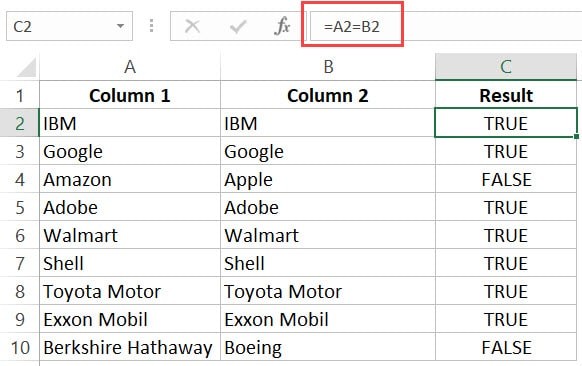
1.1. Exact Row Comparison
This method involves comparing cells in the same row across two columns. It’s straightforward and useful for verifying data integrity.
How to Do It:
-
Using the “=” Operator:
- In a new column, enter the formula
=A2=B2(assuming your data starts in row 2). - Drag the formula down to apply it to all rows.
- The result will be
TRUEif the values in columns A and B match, andFALSEif they don’t.
- In a new column, enter the formula
-
Using the IF Function:
- For a more descriptive result, use the formula
=IF(A2=B2,"Match","Mismatch"). - This will return “Match” if the values are the same and “Mismatch” if they differ.
- For a more descriptive result, use the formula
-
Case-Sensitive Comparison:
- To perform a case-sensitive comparison, use the
EXACTfunction within anIFformula:=IF(EXACT(A2,B2),"Match","Mismatch"). - This ensures that “IBM” and “ibm” are treated as different values.
- To perform a case-sensitive comparison, use the
1.2. Conditional Formatting
Conditional formatting is a powerful tool for visually highlighting matches or differences between two columns.
How to Highlight Rows with Matching Data:
-
Select the entire dataset.
-
Go to the “Home” tab.
-
Click on “Conditional Formatting” in the “Styles” group.
-
Select “New Rule”.
-
Choose “Use a formula to determine which cells to format”.
-
Enter the formula
=$A1=$B1in the formula field. -
Click the “Format” button to specify the formatting for matching cells.
-
Click “OK”.
This will highlight all rows where the data in column A matches the data in column B.
1.3. Compare Two Columns and Highlight Matches
To highlight matching data across two columns, use the duplicate values feature in conditional formatting.
How to Do It:
-
Select the entire dataset.
-
Go to the “Home” tab.
-
Click on “Conditional Formatting”.
-
Hover over “Highlight Cell Rules”.
-
Click on “Duplicate Values”.
-
Ensure “Duplicate” is selected.
-
Specify the formatting.
-
Click “OK”.
This will highlight all matching entries in both columns.
1.4. Compare Two Columns and Highlight Mismatched Data
To highlight data points that are present in one column but not in the other, use the “Unique” values option in conditional formatting.
How to Do It:
-
Select the entire dataset.
-
Go to the “Home” tab.
-
Click on “Conditional Formatting”.
-
Hover over “Highlight Cell Rules”.
-
Click on “Duplicate Values”.
-
In the “Duplicate Values” dialog box, select “Unique”.
-
Specify the formatting.
-
Click “OK”.
This will highlight all unique entries, showing you the mismatched data.
1.5. Lookup Formulas (VLOOKUP, MATCH, INDEX)
Lookup formulas are essential for comparing data and retrieving corresponding values from one column to another.
- VLOOKUP: Searches for a value in the first column of a range and returns a value from a column to the right.
- MATCH: Searches for a value in a range and returns the relative position of that item in the range.
- INDEX: Returns a value or the reference to a value from within a table or range.
How to Use VLOOKUP to Find Missing Data Points:
=ISERROR(VLOOKUP(A2,$B$2:$B$10,1,0))This formula checks if the company name in column A is present in column B. If the VLOOKUP returns an error (#N/A), the ISERROR function returns TRUE, indicating the data is missing in column B.
How to Use MATCH to Find Missing Data Points:
=NOT(ISNUMBER(MATCH(A2,$B$2:$B$10,0)))This formula uses the MATCH function to find the position of the company name from column A in column B. If there is no match, MATCH returns an error, and ISNUMBER returns FALSE. The NOT function then inverts this to TRUE, indicating the data is missing.
1.6. Compare Two Columns and Pull the Matching Data (Exact)
To fetch matching data from one column to another based on an exact match, you can use VLOOKUP or INDEX/MATCH.
Using VLOOKUP:
=VLOOKUP(D2,$A$2:$B$14,2,0)This formula looks up the value in cell D2 within the range $A$2:$B$14 and returns the corresponding value from the second column (column B).
Using INDEX/MATCH:
=INDEX($A$2:$B$14,MATCH(D2,$A$2:$A$14,0),2)This formula first uses MATCH to find the row number where the value in cell D2 is located in the range $A$2:$A$14. Then, INDEX uses this row number to return the value from the second column of the range $A$2:$B$14.
1.7. Compare Two Columns and Pull the Matching Data (Partial)
When dealing with datasets where there are minor differences in the names or entries, you can use wildcard characters with lookup formulas to perform a partial match.
Using VLOOKUP with Wildcards:
=VLOOKUP("*"&D2&"*",$A$2:$B$14,2,0)This formula uses the asterisk (*) as a wildcard to match any characters before and after the value in cell D2.
Using INDEX/MATCH with Wildcards:
=INDEX($A$2:$B$14,MATCH("*"&D2&"*",$A$2:$A$14,0),2)This formula combines INDEX and MATCH with the asterisk wildcard to achieve a partial match.
2. How Can I Use Excel To Compare Data Sets For Inconsistencies?
Comparing datasets for inconsistencies is a crucial task in data analysis. Excel provides several functions and techniques to identify discrepancies, ensuring data accuracy and reliability. Here are some effective methods:
- Using Conditional Formatting: Highlight differences between two datasets based on specific criteria.
- Combining VLOOKUP with ISNA: Identify missing values or discrepancies between two lists.
- Employing COUNTIF: Count the occurrences of values in one dataset to check for inconsistencies in another.
- Using Array Formulas: Perform complex comparisons across multiple columns or rows to find inconsistencies.
- Leveraging the IF Function: Create custom rules to flag inconsistencies based on specific conditions.
By utilizing these methods, you can systematically compare datasets in Excel, pinpoint inconsistencies, and take corrective actions to maintain data integrity.
2.1. Using Conditional Formatting
Conditional formatting is a valuable tool for highlighting inconsistencies between two datasets, allowing you to quickly identify discrepancies.
How to Highlight Differences:
-
Select the Range: Choose the range of cells you want to compare.
-
Go to Conditional Formatting: Navigate to the “Home” tab, click on “Conditional Formatting,” and select “New Rule.”
-
Use a Formula: Choose “Use a formula to determine which cells to format.”
-
Enter the Formula:
- To highlight values in column A that are different from column B in the same row, use the formula
=$A1<>$B1. - Click “Format” to choose a highlighting style, then click “OK.”
- To highlight values in column A that are different from column B in the same row, use the formula
-
Apply the Rule: Click “OK” in the “New Formatting Rule” dialog to apply the formatting.
This will highlight all cells where the values in column A do not match the values in column B.
2.2. Combining VLOOKUP with ISNA
Combining VLOOKUP with ISNA is an effective way to identify missing values or discrepancies between two lists. This method checks if values from one list exist in another.
How to Use This Combination:
-
Set Up Your Data: Ensure you have two columns of data to compare.
-
Enter the Formula:
- In a new column, enter the formula
=ISNA(VLOOKUP(A2,B:B,1,FALSE)). - Here,
A2is the first value in column A that you want to check against column B.B:Bis the entire column B, andFALSEensures an exact match.
- In a new column, enter the formula
-
Drag the Formula: Drag the formula down to apply it to all rows in column A.
The formula returns TRUE if the value from column A is not found in column B (indicating an inconsistency) and FALSE if the value is found.
2.3. Employing COUNTIF
The COUNTIF function can be used to count the number of times a value from one dataset appears in another, helping you check for inconsistencies.
How to Use COUNTIF:
-
Set Up Your Data: Ensure you have two columns of data to compare.
-
Enter the Formula:
- In a new column, enter the formula
=COUNTIF(B:B,A2). - Here,
B:Bis the range you are checking (entire column B), andA2is the criterion (the value from column A).
- In a new column, enter the formula
-
Drag the Formula: Drag the formula down to apply it to all rows in column A.
If the result is 0, the value from column A does not appear in column B, indicating an inconsistency. If the result is greater than 0, the value appears in column B that many times.
2.4. Using Array Formulas
Array formulas allow you to perform complex comparisons across multiple columns or rows to find inconsistencies. These formulas can handle more advanced scenarios than standard formulas.
How to Use Array Formulas:
-
Select the Range: Choose the range where you want the results.
-
Enter the Formula:
- For example, to compare two ranges
A1:A10andB1:B10, enter the formula=SUM(IF(A1:A10<>B1:B10,1,0)). - This formula counts the number of cells where the values in the two ranges are different.
- For example, to compare two ranges
-
Enter as Array Formula: Press
Ctrl + Shift + Enterto enter the formula as an array formula. Excel will automatically add curly braces{}around the formula.
The result will be the number of inconsistencies between the two ranges.
2.5. Leveraging the IF Function
The IF function allows you to create custom rules to flag inconsistencies based on specific conditions. This is particularly useful when you have specific criteria for identifying inconsistencies.
How to Use the IF Function:
-
Set Up Your Data: Ensure you have the columns you want to compare.
-
Enter the Formula:
- In a new column, enter the formula
=IF(A2<>B2,"Inconsistent","Consistent"). - This formula checks if the value in
A2is different from the value inB2. If they are different, it returns “Inconsistent”; otherwise, it returns “Consistent”.
- In a new column, enter the formula
-
Drag the Formula: Drag the formula down to apply it to all rows.
This will flag each row as either “Inconsistent” or “Consistent” based on your specified condition.
3. How Do I Find Differences Between Two Lists In Excel?
Finding differences between two lists in Excel is a common task that can be accomplished using various methods. These methods help identify items that are unique to each list, ensuring data accuracy and completeness. Here are some effective techniques:
- Using Conditional Formatting with Unique Values: Highlight items that appear in only one of the lists.
- Combining VLOOKUP with ISNA: Identify items in one list that are not present in the other.
- Employing the MATCH Function: Find the position of items from one list in another, identifying missing items.
- Using the IF Function: Create a custom comparison to flag differences based on specific criteria.
- Leveraging Advanced Filter: Filter lists to show only unique items.
By employing these techniques, you can efficiently identify and manage differences between two lists in Excel, ensuring data consistency and accuracy.
3.1. Using Conditional Formatting with Unique Values
Conditional formatting can be used to highlight items that appear in only one of the lists, making it easy to visually identify differences.
How to Use Conditional Formatting:
-
Select Both Lists: Select the entire range of both lists that you want to compare.
-
Go to Conditional Formatting: Navigate to the “Home” tab, click on “Conditional Formatting,” and select “New Rule.”
-
Select Unique or Duplicate Rule: Choose “Format only unique or duplicate values.”
-
Format Unique Values: Select “unique” in the dropdown menu.
- Click “Format” to choose a highlighting style, then click “OK.”
-
Apply the Rule: Click “OK” in the “New Formatting Rule” dialog to apply the formatting.
This will highlight items that are unique to each list, showing you the differences.
3.2. Combining VLOOKUP with ISNA
Combining VLOOKUP with ISNA is an effective method to identify items in one list that are not present in the other.
How to Use This Combination:
-
Set Up Your Data: Ensure you have two columns of data to compare.
-
Enter the Formula:
- In a new column next to the first list, enter the formula
=ISNA(VLOOKUP(A2,B:B,1,FALSE)). - Here,
A2is the first value in column A that you want to check against column B.B:Bis the entire column B, andFALSEensures an exact match.
- In a new column next to the first list, enter the formula
-
Drag the Formula: Drag the formula down to apply it to all rows in column A.
The formula returns TRUE if the value from column A is not found in column B (indicating a difference) and FALSE if the value is found.
3.3. Employing the MATCH Function
The MATCH function can be used to find the position of items from one list in another, helping you identify missing items.
How to Use the MATCH Function:
-
Set Up Your Data: Ensure you have two columns of data to compare.
-
Enter the Formula:
- In a new column next to the first list, enter the formula
=ISERROR(MATCH(A2,B:B,0)). - Here,
A2is the first value in column A that you want to check against column B.B:Bis the entire column B, and0ensures an exact match.
- In a new column next to the first list, enter the formula
-
Drag the Formula: Drag the formula down to apply it to all rows in column A.
The formula returns TRUE if the value from column A is not found in column B (indicating a difference) and FALSE if the value is found.
3.4. Using the IF Function
The IF function allows you to create a custom comparison to flag differences based on specific criteria. This is particularly useful when you have specific conditions for identifying differences.
How to Use the IF Function:
-
Set Up Your Data: Ensure you have the columns you want to compare.
-
Enter the Formula:
- In a new column, enter the formula
=IF(ISERROR(MATCH(A2,B:B,0)),"Unique to List 1","Common"). - This formula checks if the value in
A2is found in column B. If it’s not found, it returns “Unique to List 1”; otherwise, it returns “Common”.
- In a new column, enter the formula
-
Drag the Formula: Drag the formula down to apply it to all rows.
This will flag each item as either “Unique to List 1” or “Common” based on your specified condition.
3.5. Leveraging Advanced Filter
Advanced Filter can be used to filter lists to show only unique items, making it easy to identify differences between two lists.
How to Use Advanced Filter:
-
Copy Lists: Copy both lists into a single column.
-
Select Data Tab: Go to the “Data” tab on the Excel ribbon.
-
Click Advanced: In the “Sort & Filter” group, click “Advanced.”
-
Set Up Advanced Filter:
- Action: Choose “Copy to another location.”
- List range: Select the range of your combined list.
- Criteria range: Leave this blank.
- Copy to: Select a cell where you want the filtered list to start.
- Unique records only: Check this box.
-
Click OK: Excel will copy the unique items to the specified location.
This will give you a list of items that appear only once, showing you the differences between the two original lists.
4. Can Excel Highlight Duplicate Values In Two Columns?
Yes, Excel can highlight duplicate values in two columns using conditional formatting. This feature helps you quickly identify entries that are present in both columns, making it easier to manage and analyze your data. Here’s how you can do it:
- Using Conditional Formatting: Highlight duplicate values across two columns.
- Customizing the Highlighting: Adjust the formatting to suit your needs.
- Applying to Multiple Columns: Extend the formatting to more than two columns if necessary.
By following these steps, you can efficiently highlight and manage duplicate values in your Excel spreadsheets, ensuring data accuracy and consistency.
4.1. Using Conditional Formatting
Conditional formatting is a straightforward method to highlight duplicate values across two columns.
How to Use Conditional Formatting:
-
Select Both Columns: Select the entire range of both columns that you want to compare.
-
Go to Conditional Formatting: Navigate to the “Home” tab, click on “Conditional Formatting,” and select “Highlight Cells Rules.”
-
Select Duplicate Values: Choose “Duplicate Values” from the dropdown menu.
-
Choose Formatting:
- In the “Duplicate Values” dialog, you can choose the formatting style you want to apply to the duplicate values (e.g., light red fill, yellow fill, etc.).
- Click “OK” to apply the formatting.
Excel will now highlight all duplicate values that appear in both columns.
4.2. Customizing the Highlighting
You can customize the highlighting style to make the duplicate values stand out more clearly.
How to Customize Highlighting:
-
Follow Steps 1-3 Above: Perform the initial steps for using conditional formatting.
-
Custom Format:
- In the “Duplicate Values” dialog, click on the dropdown menu next to “with” and select “Custom Format.”
- This opens the “Format Cells” dialog where you can customize the font, border, and fill.
-
Choose Your Style:
- Select the “Fill” tab to choose a background color, the “Font” tab to change the font style and color, and the “Border” tab to add a border.
- Click “OK” to save your custom format.
-
Apply the Formatting: Click “OK” in the “Duplicate Values” dialog to apply the custom formatting.
Now, Excel will highlight the duplicate values with your specified custom style.
4.3. Applying to Multiple Columns
If you need to highlight duplicate values across more than two columns, you can easily extend the conditional formatting.
How to Apply to Multiple Columns:
- Select All Columns: Select the entire range of all the columns you want to compare.
- Go to Conditional Formatting: Navigate to the “Home” tab, click on “Conditional Formatting,” and select “Highlight Cells Rules.”
- Select Duplicate Values: Choose “Duplicate Values” from the dropdown menu.
- Apply Formatting: Ensure that the formatting is set as desired, and click “OK.”
Excel will now highlight all duplicate values that appear in any of the selected columns.
5. How Can I Compare Two Excel Sheets For Differences?
Comparing two Excel sheets for differences is a critical task for maintaining data consistency and accuracy. Excel provides several methods to identify discrepancies, ranging from simple techniques to more advanced formulas. Here are some effective ways to compare two Excel sheets:
- Using Conditional Formatting: Highlight cells that are different between two sheets.
- Employing VLOOKUP: Find values in one sheet that are missing or different in another.
- Combining IF and EXACT Functions: Perform case-sensitive comparisons and flag differences.
- Using Array Formulas: Compare entire ranges of cells and identify discrepancies.
- Leveraging the Inquire Add-In: Compare entire workbooks for detailed differences (available in some Excel versions).
By using these methods, you can systematically compare two Excel sheets, identify differences, and ensure data integrity.
5.1. Using Conditional Formatting
Conditional formatting is a simple way to highlight cells that are different between two Excel sheets.
How to Use Conditional Formatting:
-
Select the Range: Select the range of cells in the first sheet that you want to compare.
-
Go to Conditional Formatting: Navigate to the “Home” tab, click on “Conditional Formatting,” and select “New Rule.”
-
Use a Formula: Choose “Use a formula to determine which cells to format.”
-
Enter the Formula:
- To highlight values in Sheet1 that are different from Sheet2, use the formula
=A1<>Sheet2!A1. - Here,
A1refers to the first cell in Sheet1, andSheet2!A1refers to the corresponding cell in Sheet2.
- To highlight values in Sheet1 that are different from Sheet2, use the formula
-
Choose Formatting: Click “Format” to choose a highlighting style, then click “OK.”
-
Apply the Rule: Click “OK” in the “New Formatting Rule” dialog to apply the formatting.
Repeat these steps for Sheet2, but modify the formula to =A1<>Sheet1!A1 to highlight differences in Sheet2.
5.2. Employing VLOOKUP
VLOOKUP can be used to find values in one sheet that are missing or different in another sheet.
How to Use VLOOKUP:
-
Select a Sheet: Choose the sheet where you want to display the comparison results.
-
Enter the Formula:
- In a new column, enter the formula
=IF(ISNA(VLOOKUP(A2,Sheet2!A:B,2,FALSE)),"Missing","Different"). - Here,
A2is the first value in the first sheet that you want to check against the second sheet.Sheet2!A:Bis the range in the second sheet (assuming the comparison value is in column A and the corresponding value is in column B).
- In a new column, enter the formula
-
Drag the Formula: Drag the formula down to apply it to all rows in the first sheet.
The formula returns “Missing” if the value from the first sheet is not found in the second sheet and “Different” if the values are different.
5.3. Combining IF and EXACT Functions
Combining the IF and EXACT functions allows you to perform case-sensitive comparisons and flag differences between two sheets.
How to Use This Combination:
-
Select a Sheet: Choose the sheet where you want to display the comparison results.
-
Enter the Formula:
- In a new column, enter the formula
=IF(EXACT(A2,Sheet2!A2),"Match","Mismatch"). - Here,
A2is the first value in the first sheet that you want to check against the second sheet.Sheet2!A2is the corresponding cell in the second sheet.
- In a new column, enter the formula
-
Drag the Formula: Drag the formula down to apply it to all rows in the first sheet.
The formula returns “Match” if the values in both sheets are identical (including case) and “Mismatch” if they are different.
5.4. Using Array Formulas
Array formulas can compare entire ranges of cells and identify discrepancies between two sheets.
How to Use Array Formulas:
-
Select the Range: Choose the range where you want the results.
-
Enter the Formula:
- For example, to compare the ranges
Sheet1!A1:A10andSheet2!A1:A10, enter the formula=SUM(IF(Sheet1!A1:A10<>Sheet2!A1:A10,1,0)). - This formula counts the number of cells where the values in the two ranges are different.
- For example, to compare the ranges
-
Enter as Array Formula: Press
Ctrl + Shift + Enterto enter the formula as an array formula. Excel will automatically add curly braces{}around the formula.
The result will be the number of differences between the two ranges.
5.5. Leveraging the Inquire Add-In
The Inquire add-in is a powerful tool for comparing entire workbooks for detailed differences. It is available in some versions of Excel (usually professional or enterprise editions).
How to Use the Inquire Add-In:
-
Enable the Add-In:
- Go to “File” > “Options” > “Add-Ins.”
- In the “Manage” dropdown, select “COM Add-ins” and click “Go.”
- Check the box next to “Inquire” and click “OK.”
-
Compare Files:
- In the “Inquire” tab, click “Compare Files.”
- Select the two Excel files you want to compare.
-
Review Results:
- The Inquire add-in will generate a detailed report of all differences between the two files, including cell values, formulas, and formatting.
This provides a comprehensive comparison, highlighting every difference between the two workbooks.
6. What Excel Functions Can Be Used For Data Matching?
Excel offers a range of functions that are invaluable for data matching, allowing you to compare, identify, and extract relevant information from datasets. These functions can be used individually or in combination to address various data-matching needs. Here are some key Excel functions for data matching:
- VLOOKUP: Searches for a value in the first column of a range and returns a value from a column to the right.
- INDEX and MATCH: A powerful combination that can perform more flexible lookups than VLOOKUP.
- MATCH: Searches for a value in a range and returns the relative position of that item in the range.
- COUNTIF and COUNTIFS: Count the number of cells within a range that meet a given criterion or multiple criteria.
- IF: Performs a logical test and returns one value if the test is TRUE and another value if the test is FALSE.
- EXACT: Compares two text strings and returns TRUE if they are exactly the same, including case.
- FIND and SEARCH: Locate the starting position of one text string within another (FIND is case-sensitive, SEARCH is not).
By mastering these functions, you can effectively perform data matching tasks in Excel, ensuring accuracy and extracting valuable insights from your data.
6.1. VLOOKUP
VLOOKUP is one of the most commonly used functions for data matching. It searches for a value in the first column of a range and returns a value from a column to the right.
How to Use VLOOKUP:
=VLOOKUP(lookup_value, table_array, col_index_num, [range_lookup])- lookup_value: The value you want to search for.
- table_array: The range in which to search.
- col_index_num: The column number in the range from which to return a value.
- range_lookup:
TRUEfor approximate match (default),FALSEfor exact match.
Example:
To find the price of a product in a table, use VLOOKUP to search for the product name in the first column of the table and return the price from the second column.
6.2. INDEX and MATCH
The combination of INDEX and MATCH is a powerful alternative to VLOOKUP, offering more flexibility and efficiency. MATCH finds the position of a value in a range, and INDEX returns the value at that position in another range.
How to Use INDEX and MATCH:
=INDEX(array, MATCH(lookup_value, lookup_array, [match_type]))- array: The range from which to return a value.
- lookup_value: The value you want to search for.
- lookup_array: The range in which to search.
- match_type:
0for exact match,1for less than,-1for greater than.
Example:
To find the price of a product using INDEX and MATCH, use MATCH to find the row number of the product name and then use INDEX to return the price from that row in the price column.
6.3. MATCH
The MATCH function searches for a value in a range and returns the relative position of that item in the range.
How to Use MATCH:
=MATCH(lookup_value, lookup_array, [match_type])- lookup_value: The value you want to search for.
- lookup_array: The range in which to search.
- match_type:
0for exact match,1for less than,-1for greater than.
Example:
To find the row number of a specific customer in a list of customers, use MATCH with a match_type of 0 for an exact match.
6.4. COUNTIF and COUNTIFS
COUNTIF and COUNTIFS count the number of cells within a range that meet a given criterion or multiple criteria.
How to Use COUNTIF:
=COUNTIF(range, criteria)- range: The range in which to count cells.
- criteria: The condition that determines which cells to count.
How to Use COUNTIFS:
=COUNTIFS(criteria_range1, criteria1, [criteria_range2, criteria2], ...)- criteria_range1: The first range in which to evaluate criteria.
- criteria1: The condition that determines which cells to count in the first range.
- criteria_range2, criteria2, …: Additional ranges and their criteria.
Example:
To count the number of times a specific product appears in a list of products, use COUNTIF. To count the number of orders that meet specific criteria (e.g., product type and order date), use COUNTIFS.
6.5. IF
The IF function performs a logical test and returns one value if the test is TRUE and another value if the test is FALSE.
How to Use IF:
=IF(logical_test, value_if_true, value_if_false)- logical_test: The condition to evaluate.
- value_if_true: The value to return if the condition is TRUE.
- value_if_false: The value to return if the condition is FALSE.
Example:
To check if a sale amount is greater than a target amount, use IF to return “Achieved” if