How To Compare Two Columns In Excel For Duplicate Values is a common need for data analysis and cleaning. At COMPARE.EDU.VN, we provide various methods to identify these duplicates, from basic formulas to more advanced techniques. This article will guide you through several approaches to effectively compare two columns, ensuring your data is accurate and reliable. Learn how to compare data, find matching entries, and highlight differences using Excel’s versatile features.
1. Understanding the Basics of Comparing Columns in Excel
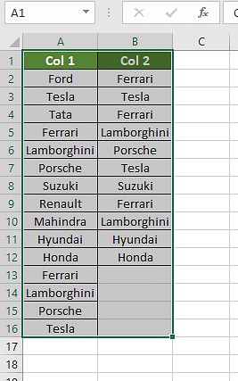
Comparing columns in Excel involves checking corresponding cells in two or more columns to identify similarities, differences, or duplicates. This process is essential for data validation, cleaning, and analysis. Whether you’re comparing lists of names, product IDs, or financial data, Excel offers several tools to streamline the comparison. Understanding the basic techniques, such as conditional formatting and simple formulas, is the first step toward mastering this skill. These methods allow you to quickly spot discrepancies and ensure data integrity.
2. Why Compare Columns in Excel?
There are numerous reasons why you might need to compare columns in Excel:
- Data Validation: Ensure data accuracy by comparing entries across different columns.
- Duplicate Identification: Find and remove duplicate entries to clean your data.
- Data Integration: Verify data consistency when merging data from different sources.
- Error Detection: Identify errors or inconsistencies in your datasets.
- Reporting: Highlight matching or differing data for reports and presentations.
- List Management: Compare lists to find missing or extra items.
- Financial Analysis: Ensure financial records match across different reports.
3. Methods for Comparing Two Columns in Excel
Excel provides several methods to compare two columns, each with its own strengths and weaknesses. Here are some of the most effective techniques:
- Conditional Formatting: Highlight duplicate or unique values.
- Equals Operator (=): Compare individual cells for matches.
- VLOOKUP Function: Find matches in one column based on values in another.
- IF Formula: Display custom messages for matches and differences.
- EXACT Formula: Perform case-sensitive comparisons.
- COUNTIF Function: Count the number of times a value appears in a column.
- MATCH Function: Find the position of a value in a column.
- INDEX and MATCH Functions: Retrieve matching data from another column.
4. Using Conditional Formatting to Highlight Duplicates
Conditional formatting is a quick and visual way to compare two columns for duplicate values. Here’s how to use it:
4.1. Step 1: Select the Columns
Select both columns you want to compare. Click on the column header (e.g., A, B) to select the entire column.
4.2. Step 2: Open Conditional Formatting
Go to the “Home” tab on the Excel ribbon. Click on “Conditional Formatting” in the “Styles” group.
4.3. Step 3: Highlight Duplicate Values
From the dropdown menu, choose “Highlight Cells Rules” and then select “Duplicate Values.”
4.4. Step 4: Choose a Formatting Style
In the “Duplicate Values” dialog box, you can choose a formatting style (e.g., light red fill with dark red text). Click “OK.”
Excel will now highlight all duplicate values in the selected columns, making them easy to identify.
4.5. Customizing the Highlight
You can customize the highlight color and style by clicking on “Custom Format” in the “Duplicate Values” dialog box. This allows you to choose a specific fill color, font style, or border.
5. Comparing Columns with the Equals Operator (=)
The equals operator (=) is a simple way to compare individual cells in two columns. This method is best for a quick, row-by-row comparison.
5.1. Step 1: Create a Result Column
Create a new column next to the columns you want to compare (e.g., Column C).
5.2. Step 2: Enter the Formula
In the first cell of the result column (e.g., C2), enter the formula =A2=B2. This formula compares the value in cell A2 with the value in cell B2.
5.3. Step 3: Drag the Formula Down
Drag the formula down to apply it to all rows in your data. Excel will return “TRUE” for matching cells and “FALSE” for differing cells.
5.4. Using IF to Customize Results
You can use the IF formula to display custom messages instead of “TRUE” and “FALSE.” For example, the formula =IF(A2=B2, "Match", "No Match") will display “Match” if the cells are identical and “No Match” if they are different.
6. Utilizing the VLOOKUP Function
VLOOKUP is a powerful function for finding matches in one column based on values in another. It’s particularly useful when you want to check if a value from one column exists in another column.
6.1. Understanding the VLOOKUP Syntax
The syntax for VLOOKUP is:
=VLOOKUP(lookup_value, table_array, col_index_num, [range_lookup])
lookup_value: The value you want to search for.table_array: The range of cells where you want to search for the lookup value.col_index_num: The column number in the table array from which to return a value.[range_lookup]: An optional argument that specifies whether to find an exact match (FALSE) or an approximate match (TRUE).
6.2. Step 1: Create a Result Column
Create a new column where you want to display the results of the VLOOKUP function.
6.3. Step 2: Enter the VLOOKUP Formula
In the first cell of the result column, enter the VLOOKUP formula. For example, if you want to check if the values in column A exist in column B, you can use the formula:
=VLOOKUP(A2, B:B, 1, FALSE)
This formula searches for the value in cell A2 in column B. If a match is found, it returns the value from the first column of the table array (in this case, column B itself). If no match is found, it returns an error.
6.4. Step 3: Handle Errors with IFERROR
To handle errors when no match is found, you can use the IFERROR function. The IFERROR function allows you to display a custom message when VLOOKUP returns an error. For example:
=IFERROR(VLOOKUP(A2, B:B, 1, FALSE), "Not Found")
This formula will display “Not Found” if the value in A2 is not found in column B.
6.5. Step 4: Drag the Formula Down
Drag the formula down to apply it to all rows in your data. The result column will now show the matching values or “Not Found” for each row.
7. Using the IF Formula for Custom Comparisons
The IF formula allows you to create custom comparisons based on specific criteria. This is particularly useful when you want to display different results depending on whether the values match or not.
7.1. Understanding the IF Syntax
The syntax for the IF formula is:
=IF(logical_test, value_if_true, value_if_false)
logical_test: The condition you want to evaluate.value_if_true: The value to return if the condition is true.value_if_false: The value to return if the condition is false.
7.2. Step 1: Create a Result Column
Create a new column where you want to display the results of the IF formula.
7.3. Step 2: Enter the IF Formula
In the first cell of the result column, enter the IF formula. For example, to compare the values in columns A and B and display “Match” if they are the same and “Different” if they are not, use the formula:
=IF(A2=B2, "Match", "Different")
7.4. Step 3: Drag the Formula Down
Drag the formula down to apply it to all rows in your data. The result column will now show “Match” or “Different” for each row, based on the comparison of the values in columns A and B.
7.5. Advanced IF Conditions
You can use more complex logical tests in the IF formula by combining multiple conditions with the AND and OR functions. For example, to check if both columns A and B are equal and column C is greater than 10, you can use the formula:
=IF(AND(A2=B2, C2>10), "Condition Met", "Condition Not Met")
8. Performing Case-Sensitive Comparisons with the EXACT Formula
The EXACT formula compares two strings and returns TRUE if they are exactly the same, including case. This is useful when you need to differentiate between “Apple” and “apple.”
8.1. Understanding the EXACT Syntax
The syntax for the EXACT formula is:
=EXACT(text1, text2)
text1: The first text string to compare.text2: The second text string to compare.
8.2. Step 1: Create a Result Column
Create a new column where you want to display the results of the EXACT formula.
8.3. Step 2: Enter the EXACT Formula
In the first cell of the result column, enter the EXACT formula. For example, to compare the values in cells A2 and B2, use the formula:
=EXACT(A2, B2)
8.4. Step 3: Drag the Formula Down
Drag the formula down to apply it to all rows in your data. The result column will now show “TRUE” if the values are exactly the same (including case) and “FALSE” if they are different.
9. Counting Matches with the COUNTIF Function
The COUNTIF function counts the number of cells within a range that meet a given criterion. This can be useful for finding out how many times a specific value from one column appears in another column.
9.1. Understanding the COUNTIF Syntax
The syntax for the COUNTIF formula is:
=COUNTIF(range, criteria)
range: The range of cells you want to count.criteria: The condition that determines which cells to count.
9.2. Step 1: Create a Result Column
Create a new column where you want to display the results of the COUNTIF function.
9.3. Step 2: Enter the COUNTIF Formula
In the first cell of the result column, enter the COUNTIF formula. For example, to count how many times the value in cell A2 appears in column B, use the formula:
=COUNTIF(B:B, A2)
9.4. Step 3: Drag the Formula Down
Drag the formula down to apply it to all rows in your data. The result column will now show the number of times each value from column A appears in column B.
10. Finding the Position of a Value with the MATCH Function
The MATCH function searches for a specified item in a range of cells and returns the relative position of that item in the range. This can be helpful for determining where a value from one column appears in another.
10.1. Understanding the MATCH Syntax
The syntax for the MATCH formula is:
=MATCH(lookup_value, lookup_array, [match_type])
lookup_value: The value you want to search for.lookup_array: The range of cells you want to search in.[match_type]: An optional argument that specifies how to match the lookup value. 0 for exact match, 1 for less than, and -1 for greater than.
10.2. Step 1: Create a Result Column
Create a new column where you want to display the results of the MATCH function.
10.3. Step 2: Enter the MATCH Formula
In the first cell of the result column, enter the MATCH formula. For example, to find the position of the value in cell A2 in column B, use the formula:
=MATCH(A2, B:B, 0)
10.4. Step 3: Handle Errors with IFERROR
To handle errors when no match is found, you can use the IFERROR function. For example:
=IFERROR(MATCH(A2, B:B, 0), "Not Found")
10.5. Step 4: Drag the Formula Down
Drag the formula down to apply it to all rows in your data. The result column will now show the position of each value from column A in column B, or “Not Found” if the value is not present.
11. Combining INDEX and MATCH for Advanced Lookups
The INDEX and MATCH functions can be combined to perform more flexible and powerful lookups than VLOOKUP. This combination allows you to retrieve data from a column based on a match in another column, without being restricted by the column order.
11.1. Understanding the INDEX Syntax
The syntax for the INDEX formula is:
=INDEX(array, row_num, [column_num])
array: The range of cells from which to return a value.row_num: The row number in the array from which to return a value.[column_num]: An optional argument that specifies the column number in the array from which to return a value.
11.2. Step 1: Create a Result Column
Create a new column where you want to display the results of the INDEX and MATCH functions.
11.3. Step 2: Enter the INDEX and MATCH Formula
In the first cell of the result column, enter the formula. For example, if you want to retrieve the corresponding value from column C based on a match between column A and column B, use the formula:
=INDEX(C:C, MATCH(A2, B:B, 0))
This formula searches for the value in cell A2 in column B, and then returns the corresponding value from column C.
11.4. Step 3: Handle Errors with IFERROR
To handle errors when no match is found, you can use the IFERROR function. For example:
=IFERROR(INDEX(C:C, MATCH(A2, B:B, 0)), "Not Found")
11.5. Step 4: Drag the Formula Down
Drag the formula down to apply it to all rows in your data. The result column will now show the corresponding values from column C based on the matches between column A and column B, or “Not Found” if no match is found.
12. Comparing Multiple Columns
While most of the above methods focus on comparing two columns, you can extend them to compare multiple columns. For example, you can use conditional formatting to highlight duplicate values across multiple columns, or use the IF formula with AND/OR conditions to compare values in multiple columns simultaneously.
12.1. Conditional Formatting for Multiple Columns
To highlight duplicate values across multiple columns, select all the columns you want to compare and then use the conditional formatting rule for duplicate values.
12.2. IF Formula with AND/OR Conditions
To compare values in multiple columns using the IF formula, use the AND and OR functions to combine multiple conditions. For example, to check if columns A, B, and C are all equal, use the formula:
=IF(AND(A2=B2, B2=C2), "All Match", "Not All Match")
13. Best Practices for Comparing Columns in Excel
- Clean Your Data: Before comparing columns, ensure that your data is clean and consistent. Remove any leading or trailing spaces, correct any typos, and standardize the format of your data.
- Use Absolute References: When using formulas like VLOOKUP and COUNTIF, use absolute references (e.g.,
$B$2:$B$10) to prevent the range from changing when you drag the formula down. - Test Your Formulas: Always test your formulas on a small sample of your data to ensure that they are working correctly before applying them to the entire dataset.
- Handle Errors: Use the IFERROR function to handle errors gracefully and display meaningful messages instead of error codes.
- Document Your Work: Add comments to your formulas and spreadsheets to explain what each formula does and why you are using it.
- Use Named Ranges: For complex formulas, use named ranges to make your formulas easier to read and understand.
14. Real-World Scenarios and Examples
14.1. Scenario 1: Comparing Customer Lists
Imagine you have two lists of customer names in columns A and B. You want to identify which customers are present in both lists. You can use the VLOOKUP function to check if each name in column A exists in column B, and display “Found” if the name is present and “Not Found” if it is not.
14.2. Scenario 2: Verifying Product IDs
You have a list of product IDs in column A and a list of valid product IDs in column B. You want to ensure that all product IDs in column A are valid. You can use the VLOOKUP function to check if each product ID in column A exists in column B, and display “Valid” if the ID is present and “Invalid” if it is not.
14.3. Scenario 3: Comparing Financial Data
You have two sets of financial data in columns A and B. You want to ensure that the values in each row are consistent. You can use the IF formula to compare the values in each row and display “Match” if the values are the same and “Mismatch” if they are different.
15. Optimizing Your Excel Skills with COMPARE.EDU.VN
Comparing columns in Excel is a fundamental skill for data analysis and management. By mastering these techniques, you can ensure data accuracy, identify duplicates, and make informed decisions based on reliable information. At COMPARE.EDU.VN, we provide comprehensive guides and resources to help you optimize your Excel skills and tackle complex data challenges. Whether you’re a beginner or an experienced user, our platform offers valuable insights and practical tips to enhance your data analysis capabilities.
16. Frequently Asked Questions (FAQs)
16.1. How can I compare two columns in Excel for duplicate values?
You can use conditional formatting to highlight duplicate values in two columns. Select the columns, go to “Conditional Formatting,” choose “Highlight Cells Rules,” and then select “Duplicate Values.”
16.2. Is it possible to compare two columns in Excel using the INDEX-MATCH function?
Yes, you can compare two columns using the INDEX and MATCH functions. This combination allows you to retrieve data from one column based on a match in another column.
16.3. How do I compare multiple columns in Excel?
To compare multiple columns, you can use conditional formatting, IF formulas with AND/OR conditions, or combine multiple VLOOKUP functions.
16.4. How can I compare two lists in Excel for matches and differences?
You can use the VLOOKUP function to find matches between two lists. To identify differences, you can use the COUNTIF function to check if each value in one list exists in the other list.
16.5. How do I compare two columns in Excel and highlight the duplicates?
Select the two columns you want to compare, go to “Conditional Formatting,” choose “Highlight Cells Rules,” and select “Duplicate Values.” Choose a formatting style to highlight the duplicates.
16.6. What is the EXACT formula used for?
The EXACT formula is used for case-sensitive comparisons. It returns TRUE if two text strings are exactly the same, including case, and FALSE if they are different.
16.7. How do I use the IF formula to compare two columns?
Enter the formula =IF(A2=B2, "Match", "Different") in a result column. This will display “Match” if the values in A2 and B2 are the same and “Different” if they are not.
16.8. Can I use VLOOKUP to compare two columns?
Yes, you can use VLOOKUP to compare two columns. The formula =VLOOKUP(A2, B:B, 1, FALSE) checks if the value in A2 exists in column B and returns the value from column B if a match is found.
16.9. How can I handle errors when using VLOOKUP to compare columns?
Use the IFERROR function to handle errors. For example, =IFERROR(VLOOKUP(A2, B:B, 1, FALSE), "Not Found") will display “Not Found” if no match is found.
16.10. What are some best practices for comparing columns in Excel?
Best practices include cleaning your data, using absolute references, testing your formulas, handling errors, and documenting your work.
17. Take the Next Step with COMPARE.EDU.VN
Mastering the art of comparing columns in Excel is essential for anyone working with data. Whether you are cleaning data, identifying duplicates, or verifying data consistency, the techniques outlined in this guide will help you streamline your workflow and improve your accuracy.
Ready to take your data analysis skills to the next level? Visit COMPARE.EDU.VN today to explore more tutorials, guides, and resources. Our platform offers a wealth of information to help you become a data analysis expert.
Contact Us:
- Address: 333 Comparison Plaza, Choice City, CA 90210, United States
- WhatsApp: +1 (626) 555-9090
- Website: COMPARE.EDU.VN
Discover the power of data comparison and make smarter decisions with COMPARE.EDU.VN.
Unlock the potential of Excel and transform your data analysis skills today. At compare.edu.vn, we are committed to providing you with the tools and knowledge you need to succeed. Start your journey now and become a data comparison pro.