Comparing two columns in Excel and highlighting differences is a common task, and at COMPARE.EDU.VN, we provide the solutions needed to identify matches and discrepancies efficiently. Our comprehensive guide offers diverse methods, from simple formulas to advanced tools, ensuring you can effectively analyze your data. Discover how to quickly compare lists, find unique entries, and highlight matches for clear data insights.
1. What is the Easiest Way to Compare Two Columns in Excel?
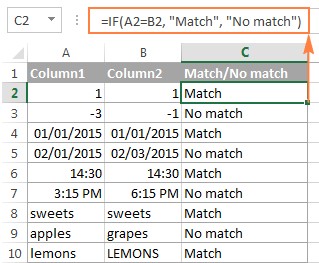
The easiest way to compare two columns in Excel involves using the IF function. This method allows you to quickly identify matches or differences between corresponding cells in two columns.
To compare two columns row by row, utilize the IF formula. In a new column, enter the formula comparing the first two cells (e.g., A2 and B2). Drag the fill handle to apply the formula to other rows. The formula =IF(A2=B2,"Match","") identifies matching cells, while =IF(A2<>B2,"No match","") finds differences. You can combine both into one formula like =IF(A2=B2,"Match","No match"). This method works for numbers, dates, times, and text strings. For case-sensitive comparisons, use the EXACT function, such as =IF(EXACT(A2, B2), "Match", "Unique"). This approach is straightforward and effective for basic comparisons.
2. How Do You Compare Two Columns in Excel for Differences?
To effectively compare two columns in Excel for differences, you can use a combination of the COUNTIF and IF functions. This method identifies values in one column that do not appear in another.
Use the COUNTIF function within an IF formula to search for values from column A in column B. For example, the formula =IF(COUNTIF($B:$B, $A2)=0, "No match in B", "") checks if the value in cell A2 exists in column B. If COUNTIF returns 0 (no match found), the formula displays “No match in B”; otherwise, it returns an empty string. This allows you to easily identify entries unique to column A. Alternatively, you can use the ISERROR and MATCH functions, such as =IF(ISERROR(MATCH($A2,$B$2:$B$10,0)),"No match in B",""), or an array formula like =IF(SUM(--($B$2:$B$10=$A2))=0, " No match in B", ""). These methods efficiently highlight discrepancies between the two columns.
3. How Can I Highlight Differences Between Two Columns in Excel?
Conditional formatting is a powerful tool to highlight differences between two columns in Excel. This method allows you to visually identify unique entries or mismatches.
To highlight differences, select the cells in column A, then navigate to Conditional Formatting > New Rule > Use a formula to determine which cells to format. Enter the formula =$B2<>$A2 to highlight cells in column A that do not match the corresponding values in column B. Ensure that the row reference is relative (without the $ sign) to apply the rule correctly to all rows. For highlighting unique entries in each list, use the COUNTIF function. For example, to highlight values in column A (A2:A6) that are not in column C (C2:C5), use the formula =COUNTIF($C$2:$C$5, $A2)=0. Similarly, for highlighting unique values in column C, use =COUNTIF($A$2:$A$6, $C2)=0. This approach provides a clear visual representation of the differences between the two columns.
4. What is the Best Way to Compare Multiple Columns for Matches in Excel?
The best way to compare multiple columns for matches in Excel involves using a combination of the IF function and the AND or COUNTIF functions. This approach identifies rows where all columns have the same value.
Use the IF function with the AND function to check if all cells in a row have identical values. For example, =IF(AND(A2=B2, A2=C2), "Full match", "") checks if cells A2, B2, and C2 have the same value. Alternatively, use the COUNTIF function for a more scalable solution. The formula =IF(COUNTIF($A2:$E2, $A2)=5, "Full match", "") checks if all 5 columns (A to E) in row 2 have the same value. You can also use conditional formatting to highlight these matches. Create a new rule using the formula =AND($A2=$B2, $A2=$C2) or =COUNTIF($A2:$C2, $A2)=3 (where 3 is the number of columns being compared) to highlight rows with identical values. These methods provide efficient ways to identify matches across multiple columns.
5. How Can I Use VLOOKUP to Compare Two Columns in Excel?
VLOOKUP is an effective function to compare two columns in Excel and pull matching entries from a lookup table. This method is particularly useful when you need to retrieve associated data based on matches.
Use the VLOOKUP function to compare values in one column against another and retrieve corresponding information. For example, =VLOOKUP(D2, $A$2:$B$6, 2, FALSE) compares the value in cell D2 with the values in column A (range A2:A6) and, if a match is found, retrieves the corresponding value from column B (the second column in the specified range). If no match is found, the formula returns #N/A. Alternatively, you can use the INDEX and MATCH functions, such as =INDEX($B$2:$B$6, MATCH($D2, $A$2:$A$6, 0)), or the XLOOKUP function (available in Excel 2021 and Excel 365), such as =XLOOKUP(D2, $A$2:$A$6, $B$2:$B$6). These functions offer flexible ways to compare columns and retrieve associated data based on matches.
6. How to Compare Two Columns in Excel and Show Differences Using the EXACT Function?
The EXACT function in Excel is specifically designed for comparing two text strings, taking into account case sensitivity. This makes it a valuable tool for accurately identifying differences between two columns that contain text data.
To compare two columns using the EXACT function, embed it within an IF statement. For example, use the formula =IF(EXACT(A2, B2), "Match", "No Match") to compare the text in cell A2 with the text in cell B2. If the text is an exact match, including case, the formula will return “Match”; otherwise, it will return “No Match”. This approach is particularly useful when you need to differentiate between entries that may appear similar but have different capitalization. The EXACT function ensures that only truly identical text strings are considered matches.
7. What Are Some Formula-Free Methods to Compare Two Columns in Excel?
While formulas are powerful, Excel also offers formula-free methods to compare two columns, leveraging built-in features for easier analysis.
One such method is using Conditional Formatting to highlight duplicate or unique values directly. Another approach is to use Excel’s “Remove Duplicates” feature to identify and eliminate repeated entries, leaving you with a list of unique values. For a more comprehensive solution, consider using Excel add-ins like Ablebits Ultimate Suite, which offers tools like “Compare Two Tables” for identifying matches and differences between columns without writing formulas. These formula-free methods provide efficient alternatives for users who prefer a more visual or automated approach to data comparison.
8. How to Compare Two Columns in Excel for Matches and Return a Value from a Third Column?
To compare two columns for matches and return a value from a third column, you can use the INDEX-MATCH functions or VLOOKUP, providing powerful ways to retrieve corresponding data.
Using INDEX-MATCH, the formula =INDEX(C:C, MATCH(A2, B:B, 0)) compares the value in cell A2 with the values in column B. If a match is found, the formula returns the corresponding value from column C. Similarly, with VLOOKUP, use =VLOOKUP(A2, B:C, 2, FALSE) to compare A2 with column B and return the value from column C (the second column in the range). If no match is found, VLOOKUP returns #N/A. These methods efficiently link matching entries to their associated values in another column, enabling you to retrieve and analyze related data seamlessly.
9. How Do You Find Case-Sensitive Matches When Comparing Two Columns in Excel?
Finding case-sensitive matches requires a function that distinguishes between uppercase and lowercase letters, and the EXACT function in Excel is perfect for this.
To perform a case-sensitive comparison, use the EXACT function within an IF statement. For example, the formula =IF(EXACT(A2, B2), "Match", "No Match") compares the text in cell A2 with the text in cell B2, considering case. If the text is an exact match, including capitalization, the formula returns “Match”; otherwise, it returns “No Match”. This ensures that only entries with identical text, including case, are identified as matches, providing a precise comparison.
10. How Can I Compare Two Columns in Excel and Identify Duplicates?
To compare two columns in Excel and identify duplicates, you can use conditional formatting, COUNTIF, or advanced filtering, each providing a unique way to highlight or extract repeated entries.
With conditional formatting, select the columns and create a new rule using the formula =COUNTIF($A:$A,A1)>1 to highlight duplicates in column A. The COUNTIF function can also be used in a formula like =IF(COUNTIF($B:$B, $A2)>0, "Duplicate", "") to flag duplicate entries from column A that appear in column B. For advanced filtering, select your data, go to the “Data” tab, click “Advanced,” and choose to filter the list in place or copy it to another location, selecting “Unique records only” to exclude duplicates. These methods offer versatile ways to identify and manage duplicate data in Excel.
For more in-depth comparisons and detailed analysis, visit COMPARE.EDU.VN, your ultimate resource for making informed decisions through comprehensive comparisons. At COMPARE.EDU.VN, we understand the importance of accurate data analysis. Whether you are a student, professional, or data enthusiast, our platform provides the tools and knowledge to help you compare and contrast information effectively.
Need help comparing data or making informed decisions? Contact us at:
- Address: 333 Comparison Plaza, Choice City, CA 90210, United States
- WhatsApp: +1 (626) 555-9090
- Website: COMPARE.EDU.VN
Let compare.edu.vn be your trusted partner in data comparison, helping you make confident and well-informed choices.