How To Compare Two Columns In Excel And Return Differences?

Comparing two columns in Excel and identifying differences can be a time-consuming task, especially with large datasets. At COMPARE.EDU.VN, we provide you with the knowledge and skills necessary to streamline your data analysis. Learn effective techniques, from built-in functions to conditional formatting, to efficiently compare columns and extract valuable insights, enhancing your data processing, data validation, and data integrity.

1. Why Comparing Two Columns in Excel Is Essential

Excel is a powerful tool for data storage, manipulation, and informed decision-making. Data analysts rely on it for extracting insights that drive marketing and sales strategies. Consider these points:

• Impact of Missing Data: Formulas can produce skewed results if cells lack essential information.
• Spreadsheet Scale: Large spreadsheets and interconnected datasets make manual comparison impractical.

Comparing columns allows data analysts to determine whether critical data exists within specific cells. Instead of manual reviews, Excel can automate the process and show results as TRUE/FALSE, Match/Not Match, or any other user-defined message. This makes managing and validating data significantly easier.

2. Methods for Comparing Two Columns in Excel

Depending on the specific goals, several methods can streamline comparing two columns in Excel:

• Highlighting: Use functions to highlight unique or duplicate values directly in the columns.
• Conditional Formatting and Formulas: Display unique or duplicate entries through custom formatting.
• Row-by-Row Comparison: Compare data on a row-by-row basis using simple formulas.
• LOOKUP Formulas: Use lookup functions to identify matches and differences across columns.

Each method has advantages. The choice of which to use depends on the size of the dataset and the specific requirements for matching and comparing data.

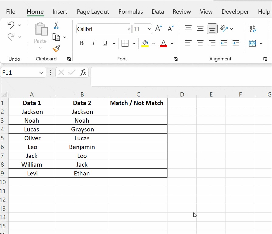
3. Comparing Two Columns with the Equals Operator

The equals operator (=) allows for straightforward, row-by-row comparisons. It flags matching data with a Match or Not Match result. The following steps are involved:

1. Formula: Use the formula =A2=B2 to compare the values in cells A2 and B2.
2. Implementation: Insert the formula in cell C2 and drag it down to apply it to subsequent rows.

The formula returns TRUE if the values match and FALSE if they differ. This method is useful for quickly identifying discrepancies between two datasets.

4. Using the IF Condition to Compare Two Columns

The IF condition in Excel extends the comparison capabilities by allowing you to specify custom results. This enables Excel to return messages like Match or Not a Match, enhancing the clarity of the comparison.

4.1. Identifying Matching Values

• Formula: Use =IF(A2=B2,"Match","") to return “Match” for matching rows and leave others blank.
• Application: Apply the formula to the desired range, and it will automatically identify matching entries.

4.2. Identifying Mismatching Values

• Formula: Use =IF(A2=B2,"Match","Not a Match") to clearly label matches and mismatches.
• Non-Equality Sign: Replace the equals sign (=) with a non-equality sign (<>) in the formula, like this: =IF(A2<>B2,"Not a Match","Match").

These adjustments make it easier to highlight where data diverges, which is essential for data validation and correction.

5. Using the EXACT() Function for Case-Sensitive Comparisons

When case sensitivity matters, the EXACT() function ensures precision by distinguishing between uppercase and lowercase text. This is particularly useful in scenarios where data accuracy is crucial, such as verifying usernames or specific codes.

• Syntax: The syntax =EXACT(text1, text2) compares two text strings exactly.
• Case Sensitivity: Unlike basic comparisons, EXACT() differentiates between “Nova Scotia” and “nova scotia”.

5.1. Practical Implementation

1. Basic Comparison: The formula =IF(A2=B2, "Match", "Mismatch") is case-insensitive and may return a false positive.
2. EXACT() Function: Using =IF(EXACT(A2, B2), "Match", "Mismatch") ensures a case-sensitive comparison.

The EXACT() function returns TRUE or FALSE, which the IF condition then uses to display “Match” or “Mismatch” accordingly. This method improves accuracy by verifying not only the content but also the case of the text.

6. Comparing Two Columns Using Conditional Formatting

Conditional formatting visually identifies duplicates or unique values without needing a third column. This is beneficial for quickly reviewing data patterns directly within your spreadsheet.

6.1. Steps to Implement Conditional Formatting

1. Access: Go to Home > Styles > Conditional Formatting.
2. Rules: Select Highlight Cell Rules > Duplicate Values.
3. Options: Choose to highlight Duplicate or Unique values.
4. Formatting: Select a formatting option, such as filling with color, changing text color, or altering cell borders.

6.2. Practical Examples

In a dataset with names in columns Data1 and Data2, conditional formatting can highlight names that appear in both columns (duplicates) or names that are unique to each column.

• Highlighting Duplicates: This helps identify common entries across the two lists.
• Highlighting Unique Values: This pinpoints entries that exist in only one list, useful for identifying missing or extra items.

6.3. Clearing Formatting

• Clear Rules: To remove conditional formatting, go to Conditional Formatting > Clear Rules > Clear Rules from Selected Cells.

Conditional formatting is advantageous for small tables, where visual cues are sufficient to grasp data patterns. However, for larger spreadsheets, more complex methods are generally needed.

7. Using Lookup Functions to Compare Two Columns

Lookup functions, such as VLOOKUP, HLOOKUP, and XLOOKUP, can search for specific values and return corresponding information from another row or column. VLOOKUP is commonly used to compare two columns and identify differences by looking for values in one column that do not appear in another.

7.1. Example Using VLOOKUP

Consider a list of exams taken by a student (Column A) and a list of subjects the student passed (Column B). You can use VLOOKUP to find which exams have not been cleared.

1. Formula: Apply the formula =VLOOKUP(A2, $B$2:$B$5, 1, 0) in cell C2.
2. Drag: Drag the formula down to apply it to all relevant cells.

The formula breaks down as follows:

• VLOOKUP(A2, $B$2:$B$5, 1, 0): Takes the value in cell A2.
• $B$2:$B$5: Compares it with values in cells B2 to B5. The dollar signs ($) create an absolute reference, preventing the range from changing when the formula is dragged.
• 1: Specifies that the comparison should be made with the first column in the specified range.
• 0: Requires an exact match.

7.2. Results

The result in Column C will show the subjects that have been cleared. Subjects not found in Column B will be marked as #N/A, indicating uncleared exams.

8. Advanced Techniques for Column Comparison

Beyond the basic methods, some advanced techniques can improve the column comparison process in Excel, especially when dealing with complex datasets.

8.1. Using the MATCH Function

The MATCH function finds the position of a specified value within a range of cells. It is useful when combined with other functions to create more sophisticated comparisons.

Example:

To check if the values in Column A exist in Column B, you can use the following formula in Column C:

=IF(ISNUMBER(MATCH(A1,B:B,0)),"Match","No Match")

• MATCH(A1,B:B,0): Searches for the value of A1 in the entire Column B. The 0 indicates an exact match.
• ISNUMBER(...): Checks if MATCH returns a number (the position of the match). If a match is found, MATCH returns the position as a number; otherwise, it returns an error.
• IF(ISNUMBER(...),"Match","No Match"): Returns “Match” if a number is returned, indicating that the value from Column A exists in Column B. Otherwise, it returns “No Match.”

8.2. Combining INDEX and MATCH

Combining INDEX and MATCH provides a more flexible and powerful alternative to VLOOKUP. This combination can look up values in a table based on both row and column criteria.

Example:

Suppose you have two tables: one with product IDs and names (Table 1) and another with product IDs and prices (Table 2). To bring the prices from Table 2 to Table 1 based on the product ID, you can use this formula in Table 1:

=INDEX(Table2[Price], MATCH(Table1[ProductID],Table2[ProductID],0))

• MATCH(Table1[ProductID],Table2[ProductID],0): Finds the row number in Table2 where the ProductID matches.
• INDEX(Table2[Price], ...): Retrieves the Price from Table2 at the matched row number.

8.3. Using Array Formulas

Array formulas can perform calculations on multiple items in an array. They are useful for complex comparisons that require evaluating multiple conditions at once.

Example:

To compare two ranges and return an array of TRUE/FALSE values indicating whether each pair of cells is equal, enter this formula as an array formula (press Ctrl + Shift + Enter):

=A1:A5=B1:B5

This formula will return an array like {TRUE;FALSE;TRUE;TRUE;FALSE}. To see the individual results, you need to enter the formula into a range of cells that matches the size of the arrays being compared.

8.4. Comparing Data Across Multiple Sheets or Workbooks

When comparing data across different sheets or workbooks, you need to reference the specific sheet or workbook in your formulas.

Example:

To compare Column A in Sheet1 with Column A in Sheet2, you can use the following formula in Sheet1:

=IF(A1=Sheet2!A1, "Match", "No Match")

• Sheet2!A1: Refers to cell A1 in Sheet2.

For comparing data between different workbooks, you need to include the workbook name in the reference:

=IF(A1=[Workbook2.xlsx]Sheet1!A1, "Match", "No Match")

• [Workbook2.xlsx]Sheet1!A1: Refers to cell A1 in Sheet1 of the Workbook2.xlsx file.

8.5. Removing Duplicates Before Comparing

Sometimes, you need to remove duplicates before comparing columns to ensure that you are comparing unique values. Excel provides a built-in feature to remove duplicates:

1. Select the Range: Select the range of cells from which you want to remove duplicates.
2. Go to Data Tab: Click on the Data tab in the Excel ribbon.
3. Remove Duplicates: Click on the Remove Duplicates button in the Data Tools group.
4. Specify Columns: In the Remove Duplicates dialog box, specify the columns that you want to check for duplicates.
5. Click OK: Click OK to remove the duplicates.

After removing duplicates, you can proceed with comparing the columns using the methods described earlier.

8.6. Using Power Query for Complex Comparisons

Power Query is a powerful data transformation and analysis tool built into Excel. It allows you to import data from various sources, clean and transform it, and perform complex comparisons.

Example:

To compare two tables and find the differences using Power Query:

1. Load Data into Power Query: Select your data ranges and go to Data > From Table/Range to load the data into the Power Query Editor.
2. Rename Queries: Rename your queries to reflect the data they contain (e.g., Table1, Table2).
3. Merge Queries:
   • Go to Home > Merge Queries.
   • Select the primary table (e.g., Table1).
   • Choose the column to match on (e.g., ProductID).
   • Select the secondary table (e.g., Table2).
   • Choose the same column to match on (e.g., ProductID).
   • Select the join kind (e.g., Left Anti, which returns rows only in the left table).
   • Click OK.
4. Expand the Merged Column: If you want to see the columns from the merged table, click the expand icon in the header of the merged column.
5. Load the Result: Go to Home > Close & Load to load the result back into your Excel worksheet.

Power Query is particularly useful for comparing large datasets or when you need to perform complex data transformations before the comparison.

9. Practical Applications of Column Comparison in Excel

Comparing columns in Excel is not just a theoretical exercise; it has numerous practical applications across various fields.

9.1. Data Validation

Data validation involves ensuring that data meets certain criteria or rules. Column comparison can be used to validate data by comparing it against a known standard or reference.

Example:

• Scenario: Verifying customer data against a master list.
• Method: Compare the customer IDs in the new data against the master list to identify any missing or incorrect entries.

9.2. Duplicate Identification

Identifying and removing duplicates is a common data cleaning task. Column comparison can help find duplicate entries within a single column or across multiple columns.

Example:

• Scenario: Removing duplicate email addresses from a mailing list.
• Method: Compare the email address column against itself to identify and remove any duplicate entries.

9.3. Reconciliation

Reconciliation involves comparing two sets of records to ensure they match. Column comparison is essential for reconciling financial data, inventory records, and other types of data.

Example:

• Scenario: Reconciling bank statements with internal accounting records.
• Method: Compare the transaction records in the bank statement against the internal records to identify any discrepancies.

9.4. Change Tracking

Column comparison can be used to track changes in data over time. By comparing two versions of a dataset, you can identify which values have been added, modified, or deleted.

Example:

• Scenario: Tracking changes in product prices over time.
• Method: Compare the current product price list against a previous version to identify any price changes.

9.5. A/B Testing Analysis

In marketing and product development, A/B testing involves comparing two versions of a product or marketing campaign to see which performs better. Column comparison can help analyze the results of A/B tests.

Example:

• Scenario: Comparing the conversion rates of two different landing pages.
• Method: Compare the conversion rate data from the two landing pages to determine which version performs better.

9.6. Reporting and Analysis

Column comparison is crucial for creating reports and conducting data analysis. By comparing different columns, you can derive insights and identify trends.

Example:

• Scenario: Analyzing sales data to identify top-performing products.
• Method: Compare the sales figures for different products to identify the top sellers.

10. Frequently Asked Questions (FAQs)

1. How do I compare two columns in Excel for differences?

To compare two columns for differences, you can use the IF function with the <> (not equal to) operator. For example, =IF(A1<>B1, "Different", "Same") will return “Different” if the values in cells A1 and B1 are not the same, and “Same” if they are the same.

2. Can I highlight the differences between two columns in Excel?

Yes, you can use conditional formatting to highlight the differences between two columns. Select the range of cells you want to compare, go to Home > Conditional Formatting > New Rule, and use a formula to determine which cells to format. For example, use the formula =A1<>B1 to highlight cells in Column A that are different from the corresponding cells in Column B.

3. How can I compare two columns and return the values that are only in one column?

You can use the VLOOKUP function or the MATCH function to compare two columns and return the values that are only in one column. For example, to find values in Column A that are not in Column B, you can use the formula =IF(ISNA(VLOOKUP(A1,B:B,1,FALSE)), A1, ""). This formula will return the value from Column A if it is not found in Column B.

4. What is the best way to compare two large columns in Excel?

For comparing large columns, using the MATCH function or Power Query can be more efficient than VLOOKUP. The MATCH function can quickly determine if a value exists in another column, and Power Query can handle large datasets more efficiently.

5. How do I compare two columns and ignore case?

To compare two columns and ignore case, you can use the UPPER or LOWER function to convert the values to the same case before comparing them. For example, =IF(UPPER(A1)=UPPER(B1), "Match", "No Match") will compare the values in cells A1 and B1, ignoring case.

6. Can I compare two columns and return the row number of the differences?

Yes, you can use the ROW function in combination with the IF function to return the row number of the differences. For example, =IF(A1<>B1, ROW(), "") will return the row number if the values in cells A1 and B1 are different.

7. How do I compare two columns with different lengths?

When comparing columns with different lengths, you need to adjust your formulas to handle the varying number of rows. You can use the IFERROR function to prevent errors when a formula tries to reference a row that does not exist. For example, =IFERROR(IF(A1=B1, "Match", "No Match"), "No Data") will return “No Data” if there is no corresponding row in one of the columns.

8. Is there a way to automatically compare two columns every time the data changes?

Yes, you can use Excel’s Worksheet_Change event to automatically compare two columns every time the data changes. You need to insert a VBA script in the worksheet’s code module that triggers the comparison whenever a cell is changed.

9. How can I compare two columns and highlight the entire row if there is a difference?

To highlight the entire row if there is a difference between two columns, you can use conditional formatting with a formula that references the entire row. Select the range of rows you want to format, go to Home > Conditional Formatting > New Rule, and use a formula like =$A1<>$B1 to highlight the entire row if the values in columns A and B are different.

10. What are some common mistakes to avoid when comparing two columns in Excel?

Some common mistakes to avoid include:

• Case Sensitivity: Forgetting to account for case sensitivity when comparing text values.
• Data Types: Comparing different data types (e.g., numbers and text) without converting them to the same type.
• Blank Cells: Not handling blank cells properly in your formulas.
• Absolute vs. Relative References: Using the wrong type of cell references, which can cause formulas to produce incorrect results when copied to other cells.

Conclusion

Comparing two columns in Excel is a fundamental skill for data analysis, validation, and manipulation. Whether you are identifying duplicates, tracking changes, or reconciling data, the methods and techniques outlined in this guide will enable you to work more efficiently and accurately.

At COMPARE.EDU.VN, we understand the importance of making informed decisions based on comprehensive data analysis. Our platform offers detailed comparisons and expert insights to help you choose the best solutions for your needs. Visit compare.edu.vn at 333 Comparison Plaza, Choice City, CA 90210, United States, or contact us via WhatsApp at +1 (626) 555-9090 for further assistance.