How To Compare Two Columns For Same Values In Excel?

Comparing two columns for the same values in Excel is a common task that can be accomplished efficiently, and COMPARE.EDU.VN can guide you through various methods to achieve this. This comprehensive guide explores various techniques, from simple formulas to built-in Excel tools, enabling you to identify similarities, differences, and discrepancies between data sets effortlessly. We will explore methods of data reconciliation, data validation, and anomaly detection with the help of Excel.

1. Understanding The Need To Compare Columns In Excel

Comparing columns in Excel involves examining corresponding cells across two or more columns to identify matches, mismatches, or unique entries. This process is crucial for various tasks, including data validation, identifying duplicates, tracking changes, and ensuring data integrity. Excel stands out as the best option for these tasks when data accuracy, consistency, and reliability are paramount.

1.1. Why Is Column Comparison Important?

Column comparison is a fundamental aspect of data analysis, enabling users to gain valuable insights and maintain data quality. Here are some key reasons why it’s important:

Data Validation: Ensuring data accuracy by comparing against a reference column, thus validating records. According to research by the Data Governance Institute in 2017, proactive data validation reduces errors by up to 30%.
Duplicate Identification: Finding and removing duplicate entries to avoid inconsistencies and inflate data volumes.
Change Tracking: Monitoring changes between different versions of a dataset to understand trends and patterns.
Data Integration: Validating successful data merging from multiple sources by identifying discrepancies.
Error Detection: Pinpointing errors or anomalies in data entry or processing, like incorrect dates or values.
Reporting and Analysis: Validating the correctness of reports by comparing data against original data sources.
Compliance: Ensuring adherence to regulatory standards by regularly validating data accuracy.
Decision Making: Providing accurate data for informed decision-making.
Data Cleaning: Identifying and rectifying errors or inconsistencies in datasets to improve data quality.
Process Improvement: Uncovering inefficiencies or bottlenecks in data processing workflows by analyzing data discrepancies.

1.2. Common Scenarios For Column Comparison

Column comparison is applicable across various domains and scenarios. Here are some common use cases:

Sales Data Analysis: Comparing sales figures from different periods to identify growth trends or performance declines.
Inventory Management: Verifying inventory levels across different warehouses or locations to ensure accurate tracking and prevent stockouts.
Financial Auditing: Validating financial records by comparing transactions against bank statements or invoices.
Customer Relationship Management (CRM): Identifying duplicate customer profiles or merging contact information from different sources.
Human Resources (HR): Matching employee data across different departments or systems to ensure data consistency and accuracy.
Marketing Campaign Analysis: Comparing marketing campaign performance across different channels or demographics to optimize strategies.
Project Management: Tracking project progress by comparing planned timelines against actual completion dates.
Research and Development (R&D): Validating experimental results by comparing data from different trials or experiments.
Manufacturing Quality Control: Ensuring product quality by comparing measurements against predefined standards.
Healthcare Data Analysis: Validating patient records by comparing medical history, diagnosis, and treatment information.

2. Methods To Compare Two Columns In Excel

Excel offers several methods to compare two columns, each with its strengths and weaknesses. Choosing the right method depends on the specific requirements of your task, such as the size of the dataset, the complexity of the comparison criteria, and the desired output format. Let’s explore some of the most effective methods:

2.1. Conditional Formatting

Conditional formatting allows you to visually highlight cells based on specific criteria. This method is ideal for quickly identifying matches, mismatches, or duplicates within a dataset.

2.1.1. Highlighting Duplicate Values

To highlight duplicate values between two columns, follow these steps:

Select the two columns: Click and drag to select the entire range of cells you want to compare.
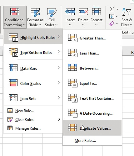
Go to Conditional Formatting: On the “Home” tab, click “Conditional Formatting” in the “Styles” group.
Choose Highlight Cells Rule: Select “Highlight Cells Rules” and then “Duplicate Values.”
Customize Formatting: In the “Duplicate Values” dialog box, choose the formatting style you want to apply to duplicate values. You can select a predefined style or create a custom format by clicking “Custom Format.”
Click OK: The duplicate values in both columns will be highlighted with the selected formatting.

2.1.2. Highlighting Unique Values

To highlight unique values between two columns, follow these steps:

Select the two columns: Click and drag to select the entire range of cells you want to compare.
Go to Conditional Formatting: On the “Home” tab, click “Conditional Formatting” in the “Styles” group.
Choose Highlight Cells Rule: Select “Highlight Cells Rules” and then “Duplicate Values.”
Change to Unique: In the “Duplicate Values” dialog box, change the selection from “Duplicate” to “Unique.”
Customize Formatting: Choose the formatting style you want to apply to unique values. You can select a predefined style or create a custom format by clicking “Custom Format.”
Click OK: The unique values in both columns will be highlighted with the selected formatting.

2.2. Using The Equals Operator (=)

The equals operator (=) provides a simple way to compare individual cells in two columns. This method is useful for identifying exact matches or mismatches between corresponding cells.

2.2.1. Comparing Individual Cells

To compare individual cells using the equals operator, follow these steps:

Create a Result Column: Insert a new column next to the columns you want to compare.
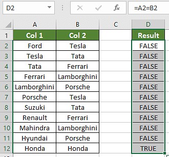
Enter the Formula: In the first cell of the result column, enter the formula =A1=B1, where A1 and B1 are the first cells in the two columns you want to compare.
Drag the Formula: Drag the fill handle (the small square at the bottom-right corner of the cell) down to apply the formula to the remaining cells in the column.
Interpret the Results: The result column will display TRUE for cells where the values in the corresponding rows of the two columns are equal, and FALSE for cells where the values are different.

2.2.2. Adding Custom Messages

To display custom messages instead of TRUE and FALSE, you can use the IF function in combination with the equals operator.

Modify the Formula: In the first cell of the result column, enter the formula =IF(A1=B1, "Match", "Mismatch"), where A1 and B1 are the first cells in the two columns you want to compare.
Drag the Formula: Drag the fill handle down to apply the formula to the remaining cells in the column.
Interpret the Results: The result column will display “Match” for cells where the values in the corresponding rows of the two columns are equal, and “Mismatch” for cells where the values are different.

2.3. VLOOKUP Function

The VLOOKUP function is a powerful tool for comparing two columns and retrieving matching data from one column based on values in another column. This method is particularly useful when you want to find corresponding values in two lists or tables.

2.3.1. Basic VLOOKUP Formula

The basic syntax of the VLOOKUP function is as follows:

=VLOOKUP(lookup_value, table_array, col_index_num, [range_lookup])

lookup_value: The value you want to search for in the first column of the table array.
table_array: The range of cells that contains the data you want to search and retrieve.
col_index_num: The column number within the table array that contains the value you want to retrieve.
[range_lookup]: An optional argument that specifies whether you want an exact match (FALSE) or an approximate match (TRUE).

2.3.2. Using VLOOKUP For Column Comparison

To use VLOOKUP to compare two columns, follow these steps:

Create a Result Column: Insert a new column next to the columns you want to compare.
Enter the Formula: In the first cell of the result column, enter the formula =VLOOKUP(A1, B:B, 1, FALSE), where A1 is the first cell in the column you want to search for, and B:B is the entire column you want to search within.
Drag the Formula: Drag the fill handle down to apply the formula to the remaining cells in the column.
Interpret the Results:
- If VLOOKUP finds a match for the lookup_value in the table_array, it will return the corresponding value from the specified col_index_num.
- If VLOOKUP does not find a match, it will return the #N/A error value.

2.3.3. Handling Errors

To handle errors and display custom messages when VLOOKUP does not find a match, you can use the IFERROR function.

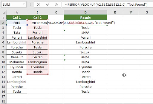
Modify the Formula: In the first cell of the result column, enter the formula =IFERROR(VLOOKUP(A1, B:B, 1, FALSE), "Not Found"), where A1 is the first cell in the column you want to search for, B:B is the entire column you want to search within, and “Not Found” is the message you want to display when no match is found.
Drag the Formula: Drag the fill handle down to apply the formula to the remaining cells in the column.
Interpret the Results: The result column will display the matching value if VLOOKUP finds a match, and “Not Found” if no match is found.

2.4. IF Formula

The IF formula allows you to perform logical comparisons between two columns and display different results based on whether the comparison is true or false. This method is useful when you want to categorize or flag data based on specific criteria.

2.4.1. Basic IF Formula

The basic syntax of the IF formula is as follows:

=IF(logical_test, value_if_true, value_if_false)

logical_test: The condition you want to evaluate.
value_if_true: The value to display if the logical_test is true.
value_if_false: The value to display if the logical_test is false.

2.4.2. Using IF For Column Comparison

To use the IF formula to compare two columns, follow these steps:

Create a Result Column: Insert a new column next to the columns you want to compare.
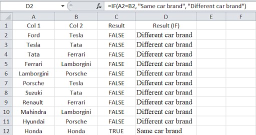
Enter the Formula: In the first cell of the result column, enter the formula =IF(A1=B1, "Same", "Different"), where A1 and B1 are the first cells in the two columns you want to compare.
Drag the Formula: Drag the fill handle down to apply the formula to the remaining cells in the column.
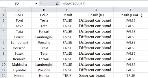
Interpret the Results: The result column will display “Same” for cells where the values in the corresponding rows of the two columns are equal, and “Different” for cells where the values are different.

2.5. EXACT Formula

The EXACT formula compares two strings and returns TRUE if they are exactly the same, including case sensitivity. This method is useful when you need to ensure that the values in two columns are identical, including capitalization and spacing.

2.5.1. Basic EXACT Formula

The basic syntax of the EXACT formula is as follows:

=EXACT(text1, text2)

text1: The first text string to compare.
text2: The second text string to compare.

2.5.2. Using EXACT For Column Comparison

To use the EXACT formula to compare two columns, follow these steps:

Create a Result Column: Insert a new column next to the columns you want to compare.
Enter the Formula: In the first cell of the result column, enter the formula =EXACT(A1, B1), where A1 and B1 are the first cells in the two columns you want to compare.
Drag the Formula: Drag the fill handle down to apply the formula to the remaining cells in the column.
Interpret the Results: The result column will display TRUE for cells where the values in the corresponding rows of the two columns are exactly the same (including case), and FALSE for cells where the values are different.

3. Choosing The Right Comparison Method

The choice of comparison method depends on the specific requirements of your task. Here’s a table summarizing the strengths and weaknesses of each method:

Method	Strengths	Weaknesses	Use Cases
Conditional Formatting	Visually highlights matches, mismatches, or duplicates; easy to set up and use.	Limited to highlighting; cannot perform calculations or retrieve data.	Quickly identifying duplicate values in a dataset; highlighting unique values for further analysis; visually flagging cells that meet specific criteria.
Equals Operator (=)	Simple and straightforward; identifies exact matches or mismatches between individual cells.	Requires manual interpretation of `TRUE` and `FALSE` results; not suitable for large datasets.	Comparing individual cells for exact matches; performing simple data validation tasks; creating custom messages using the `IF` function.
VLOOKUP Function	Retrieves matching data from one column based on values in another column; handles errors gracefully.	Can be slow for large datasets; requires careful attention to syntax and arguments.	Finding corresponding values in two lists or tables; validating data by retrieving related information; creating dynamic reports based on matching criteria.
IF Formula	Performs logical comparisons and displays different results based on whether the comparison is true or false.	Requires defining specific criteria; can become complex for nested comparisons.	Categorizing data based on specific criteria; flagging cells that meet certain conditions; creating custom messages based on logical comparisons.
EXACT Formula	Compares two strings and returns `TRUE` if they are exactly the same, including case sensitivity.	Case-sensitive; not suitable for comparing numerical values or dates.	Ensuring that the values in two columns are identical, including capitalization and spacing; validating data entry accuracy; performing case-sensitive searches.

Excel Spreadsheet Showing Column Comparison

Excel Spreadsheet with Equals Operator Comparison

4. Advanced Techniques For Column Comparison

Beyond the basic methods, Excel offers advanced techniques for column comparison that can handle more complex scenarios and provide greater flexibility. Let’s explore some of these techniques:

4.1. Comparing Multiple Columns

When you need to compare more than two columns, you can use a combination of formulas and conditional formatting to achieve the desired results. Here are a few approaches:

4.1.1. Using AND Function

The AND function returns TRUE if all conditions are true, otherwise it returns FALSE. You can use this function to compare multiple columns and check if all values in a row are the same.

Create a Result Column: Insert a new column next to the columns you want to compare.
Enter the Formula: In the first cell of the result column, enter the formula =IF(AND(A1=B1, A1=C1, B1=C1), "Match", "Mismatch"), where A1, B1, and C1 are the first cells in the three columns you want to compare.
Drag the Formula: Drag the fill handle down to apply the formula to the remaining cells in the column.
Interpret the Results: The result column will display “Match” for rows where all values are the same, and “Mismatch” for rows where at least one value is different.

4.1.2. Using COUNTIF Function

The COUNTIF function counts the number of cells within a range that meet a given criteria. You can use this function to compare multiple columns and check if all values in a row are the same.
Create a Result Column: Insert a new column next to the columns you want to compare.
Enter the Formula: In the first cell of the result column, enter the formula =IF(COUNTIF(A1:C1, A1)=3, "Match", "Mismatch"), where A1:C1 is the range of cells you want to compare, and 3 is the number of columns you are comparing.
Drag the Formula: Drag the fill handle down to apply the formula to the remaining cells in the column.
Interpret the Results: The result column will display “Match” for rows where all values are the same, and “Mismatch” for rows where at least one value is different.

4.2. Comparing Columns With Partial Matches

Sometimes, you may need to compare columns and identify partial matches, where the values are not exactly the same but share some common elements. Here are a few techniques for handling partial matches:

4.2.1. Using SEARCH Function

The SEARCH function finds the starting position of one text string within another text string. You can use this function to check if a value in one column contains a value from another column.
Create a Result Column: Insert a new column next to the columns you want to compare.
Enter the Formula: In the first cell of the result column, enter the formula =IF(ISNUMBER(SEARCH(A1, B1)), "Partial Match", "No Match"), where A1 is the value you want to search for, and B1 is the value you want to search within.
Drag the Formula: Drag the fill handle down to apply the formula to the remaining cells in the column.
Interpret the Results: The result column will display “Partial Match” for rows where the value in column A is found within the value in column B, and “No Match” for rows where the value is not found.

4.2.2. Using LEFT, RIGHT, and MID Functions

The LEFT, RIGHT, and MID functions extract a specified number of characters from the beginning, end, or middle of a text string, respectively. You can use these functions to compare specific parts of the values in two columns.
Create a Result Column: Insert a new column next to the columns you want to compare.
Enter the Formula: In the first cell of the result column, enter the formula =IF(LEFT(A1, 3)=LEFT(B1, 3), "Partial Match", "No Match"), where A1 and B1 are the values you want to compare, and 3 is the number of characters you want to extract from the left side of the strings.
Drag the Formula: Drag the fill handle down to apply the formula to the remaining cells in the column.
Interpret the Results: The result column will display “Partial Match” for rows where the first 3 characters of the values in both columns are the same, and “No Match” for rows where the characters are different.

4.3. Ignoring Case Sensitivity

As mentioned earlier, the EXACT function is case-sensitive, which means it distinguishes between uppercase and lowercase letters. If you want to compare columns while ignoring case sensitivity, you can use the following techniques:

4.3.1. Using UPPER or LOWER Functions

The UPPER function converts a text string to uppercase, while the LOWER function converts a text string to lowercase. You can use these functions to convert the values in both columns to the same case before comparing them.
Create a Result Column: Insert a new column next to the columns you want to compare.
Enter the Formula: In the first cell of the result column, enter the formula =IF(UPPER(A1)=UPPER(B1), "Match", "Mismatch"), where A1 and B1 are the values you want to compare.
Drag the Formula: Drag the fill handle down to apply the formula to the remaining cells in the column.
Interpret the Results: The result column will display “Match” for rows where the values in both columns are the same, regardless of case, and “Mismatch” for rows where the values are different.

4.4. Comparing Dates

When comparing columns containing dates, you may need to consider different date formats and potential variations in the way dates are stored. Here are a few techniques for comparing dates effectively:

4.4.1. Using DATEVALUE Function

The DATEVALUE function converts a text string representing a date to a serial number that Excel recognizes as a date. You can use this function to ensure that the dates in both columns are stored in the same format before comparing them.
Create a Result Column: Insert a new column next to the columns you want to compare.
Enter the Formula: In the first cell of the result column, enter the formula =IF(DATEVALUE(A1)=DATEVALUE(B1), "Match", "Mismatch"), where A1 and B1 are the dates you want to compare.
Drag the Formula: Drag the fill handle down to apply the formula to the remaining cells in the column.
Interpret the Results: The result column will display “Match” for rows where the dates in both columns are the same, regardless of their original format, and “Mismatch” for rows where the dates are different.

5. Best Practices For Column Comparison

To ensure accuracy and efficiency when comparing columns in Excel, follow these best practices:

Data Preparation: Clean and format your data before comparing columns to ensure consistency.
Understand Your Data: Before comparing, understand data types and inherent characteristics. This will allow you to anticipate and resolve type mismatches and inconsistencies.
Choose The Right Method: Select the comparison method that best suits your specific requirements and dataset size.
Test Your Formulas: Verify that your formulas are working correctly by testing them with sample data before applying them to the entire dataset.
Handle Errors Gracefully: Use error-handling functions like IFERROR to prevent errors from disrupting your analysis.
Document Your Steps: Keep a record of the steps you took to compare columns, including the formulas you used and the criteria you applied.
Use Named Ranges: Assign names to your ranges to improve readability and formula management.
Regularly Update Skills: Excel evolves; keep learning new features and techniques to enhance your efficiency.
Data Visualization: Where possible, use charts and graphs to represent your findings and make data easier to understand.
Backup Data: Always back up your data before performing significant data alterations.

6. Real-World Examples Of Column Comparison

Let’s explore some real-world examples of how column comparison can be used in different scenarios:

Sales Data Validation: A sales manager can compare sales data from two different systems to identify discrepancies and ensure that all sales transactions are accurately recorded.
Inventory Reconciliation: An inventory manager can compare inventory levels from two different warehouses to identify stock discrepancies and prevent stockouts.
Customer Data Cleansing: A marketing analyst can compare customer data from two different sources to identify duplicate customer profiles and merge contact information.
Financial Auditing: An auditor can compare financial data from two different periods to identify unusual transactions and ensure compliance with accounting standards.
HR Data Analysis: An HR manager can compare employee data from two different departments to identify pay disparities and ensure fair compensation practices.

7. Troubleshooting Common Issues

While comparing columns in Excel, you may encounter some common issues. Here are some troubleshooting tips to help you resolve them:

Incorrect Results: Double-check your formulas and criteria to ensure that they are accurate.
Error Values: Use error-handling functions like IFERROR to prevent errors from disrupting your analysis.
Slow Performance: Optimize your formulas and avoid using complex calculations on large datasets.
Inconsistent Formatting: Ensure that the data in both columns is formatted consistently before comparing them.
Case Sensitivity: Use the UPPER or LOWER functions to convert the values in both columns to the same case before comparing them.

8. Leveraging COMPARE.EDU.VN For Informed Decisions

Comparing columns in Excel is a valuable skill for data analysis, enabling you to identify patterns, trends, and discrepancies within your data. However, making informed decisions often requires comparing more complex options, such as products, services, or ideas. That’s where COMPARE.EDU.VN comes in.

COMPARE.EDU.VN provides comprehensive comparisons across a wide range of categories, empowering you to make informed decisions based on detailed analysis and objective evaluations. Whether you’re choosing a new software solution, selecting a healthcare provider, or evaluating investment opportunities, COMPARE.EDU.VN offers the insights you need to make the right choice.

9. Call To Action

Ready to take your data analysis skills to the next level? Visit COMPARE.EDU.VN today to explore comprehensive comparisons and make informed decisions. Whether you’re comparing products, services, or ideas, COMPARE.EDU.VN provides the insights you need to make the right choice.

Don’t rely on guesswork or incomplete information. Trust COMPARE.EDU.VN to deliver the accurate, objective comparisons you need to make confident decisions.

Contact us:

Address: 333 Comparison Plaza, Choice City, CA 90210, United States

Whatsapp: +1 (626) 555-9090

Website: compare.edu.vn

10. Frequently Asked Questions (FAQs)

10.1. How Do I Compare Two Columns In Excel For Exact Matches?

Use the EXACT function. For example, =EXACT(A1, B1) will return TRUE if A1 and B1 are exactly the same, including case.

10.2. Can I Compare Two Columns In Excel For Similar But Not Exact Matches?

Yes, use functions like SEARCH or FIND to look for one string within another. Also, consider using wildcard characters with VLOOKUP.

10.3. How Can I Highlight The Differences Between Two Columns?

Use conditional formatting with a formula like =A1<>B1 to highlight cells where the values differ.

10.4. What Is The Best Way To Compare Two Columns With Dates?

Ensure both columns are in the same date format, then use a simple =A1=B1 comparison. If formats differ, use the DATEVALUE function.

10.5. How Do I Ignore Case Sensitivity When Comparing Columns?

Use the UPPER or LOWER functions to convert both columns to the same case before comparing them. For example, =UPPER(A1)=UPPER(B1).

10.6. How Do I Compare Two Columns And Return A Value From A Third Column If There’s A Match?

Use VLOOKUP or INDEX/MATCH. For example, =VLOOKUP(A1, B:C, 2, FALSE) will return the value from column C if A1 is found in column B.

10.7. How Can I Count The Number Of Matches Between Two Columns?

Use the formula =SUMPRODUCT(--(A1:A10=B1:B10)) to count the number of matching entries in the specified ranges.

10.8. How Do I Compare Two Columns And List The Differences?

Use a combination of IF and ISNA with VLOOKUP. For example, =IF(ISNA(VLOOKUP(A1, B:B, 1, FALSE)), A1, "") will list values in column A that are not in column B.

10.9. Can I Use VBA To Compare Two Columns?

Yes, VBA can be used for more complex comparisons. A simple VBA script can loop through the columns and compare each cell.

10.10. How Do I Compare Two Columns On Different Sheets?

Reference the sheet name in your formulas. For example, =Sheet1!A1=Sheet2!A1 compares cell A1 from Sheet1 and Sheet2.