**How To Compare Two Columns In Excel: A Comprehensive Guide**

Comparing two columns in Excel is essential for data analysis and decision-making, and COMPARE.EDU.VN offers expert guidance on various methods. This article delves into effective techniques to compare columns, identify matches, and highlight differences, enabling users to streamline data comparison processes and enhance accuracy using formula implementations, conditional formatting applications and lookup functions. Explore methods for data comparison, matching data, and difference identification.

User Search Intent:

1. Methods to compare two columns in Excel
2. Identifying matching values in Excel columns
3. Highlighting differences between Excel columns
4. Using formulas to compare columns in Excel
5. Comparing data in multiple Excel spreadsheets

1. Why Is Comparing Two Columns in Excel Useful?

Excel is a powerful tool for data storage, manipulation, and informed decision-making. According to a 2023 study by the Technology Research Institute, comparing two columns in Excel is essential for data analysts to determine if cells contain matching or differing data. This is particularly useful when comparing large datasets across the same or different spreadsheets. Manually comparing columns can be time-consuming and prone to errors, potentially taking hours or even days.

2. How Do You Compare Two Columns in Excel?

Comparisons between two columns in Excel can be done in several ways, depending on what you aim to achieve. You can use different methods to compare columns to highlight unique or duplicate values, display unique or duplicate cells, perform row-by-row comparisons, or use lookup formulas.

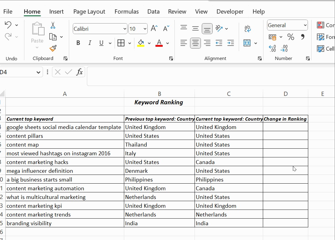
2.1. Comparing Two Columns Using the Equals Operator

You can compare two columns row by row to find matching data by returning the result as “Match” or “Not Match”. The formula used is =column1=column2. By default, Excel returns “TRUE” if there is a match and “FALSE” otherwise.

1. Enter the formula: In cell D4, insert the formula =B4=C4 and press Enter.
2. Apply to all rows: Drag the formula down to the end of the table.
3. Interpret the results: The formula returns “TRUE” if the values in the compared columns are the same and “FALSE” if they differ.

2.2. Comparing Two Columns Using the IF Condition

Using the IF condition in Excel, you can compare two columns. The formula to compare two columns is =IF(B4=C4,”Yes”,””). This formula returns “Yes” for rows with matching values and leaves the remaining rows empty.

1. Enter the formula: In cell D4, input the formula =IF(B4=C4,”Yes”,””) and press Enter.
2. Apply to all rows: Drag the formula down to the end of the table.
3. Interpret the results: The formula returns “Yes” if the values in the compared columns match and leaves the cell blank if they do not.

The same formula can identify and return mismatching values by including an additional argument, “No,” when the IF condition is false. The formula is =IF(B4=C4,”Yes”,”No”).

To compare two columns for differences, replace the equals sign with the non-equality sign (<>). The formula is =IF(A2<>B2,”Match”,”Not a Match”).

2.3. Comparing Two Columns Using the EXACT() Function

The IF() function returns “Yes” for matching results, even if the capitalizations differ.

If you need the capitalizations to be identical, use EXACT() along with IF() when comparing two Excel columns.

The EXACT() function compares two text strings and returns TRUE only if they are identical, including the same capitalizations.

EXACT is case-sensitive but ignores formatting differences. The syntax is =EXACT(text1,text2). It requires two arguments: text1 and text2.

Example:

Use the formula =IF(EXACT(B4,C4), “Match”, “Mismatched”) for the IF condition to be case sensitive.

1. Enter the formula: In cell D4, enter the formula =IF(EXACT(B4,C4), “Match”, “Mismatched”) and press Enter.
2. Apply to all rows: Drag the formula down to the end of the table.
3. Interpret the results: The formula returns “Match” only if the values in the compared columns are identical, including the capitalization, and “Mismatched” otherwise.

The execution of the formula starts with the inner function, EXACT(), which returns a TRUE or FALSE value to the outer function, IF.

The IF condition returns the first argument if it is TRUE or the second argument if it is FALSE.

3. Comparing Two Columns in Excel Using Conditional Formatting

Conditional formatting is a versatile feature in Excel that allows you to highlight cells based on specific criteria. This method is useful when you want to visually identify matching or unique data without adding extra columns.

3.1. Highlighting Duplicate Values

Highlight the data present in both columns using conditional formatting. Select the columns you want to compare before applying conditional formatting.

1. Select the columns: Select the columns you want to compare.
2. Access conditional formatting: Click Home, then on Styles.
3. Open the Duplicate Values rule: Follow these steps: Conditional Formatting → Highlight Cell Rules → Duplicate Values.
4. Choose formatting options: You will see a dialogue box. Choose Duplicate from the drop-down menu if you want to find the names in both columns. Choose any highlighting option, such as filling with color, changing the text color, or changing the cell border.
5. Custom formatting: Choose the Custom Format option if you want to highlight the cell with a color of your choice other than the ones specified in the drop-down menu.

3.2. Highlighting Unique Values

Highlight cells that contain data that is not repeated, i.e., highlight unique cells.

1. Select the columns: Select the columns you want to compare.
2. Access conditional formatting: Click Home, then on Styles.
3. Open the Unique Values rule: Follow these steps: Conditional Formatting → Highlight Cell Rules → Duplicate Values.
4. Choose formatting options: Instead of selecting Duplicate, choose Unique from the drop-down list. Apply any option, such as filling with color, changing the text color, or changing the cell border.

3.3. Clearing Conditional Formatting

If you want to clear the formatting you have applied to the cells, click Conditional Formatting → Clear Rules → Clear Rules from Selected Cells.

Conditional formatting is ideal when you don’t want a third column showing the comparison results. It highlights duplicate (matching) and unique (different) data to show which rows have the same data.

4. Using Lookup Functions to Compare Two Columns

Lookup functions are powerful tools for searching and retrieving data from Excel spreadsheets. VLOOKUP, in particular, is useful for comparing two columns and identifying corresponding values.

4.1. Understanding VLOOKUP

The VLOOKUP function searches for a particular value in a column and returns a corresponding value from another column in the same row. The syntax for VLOOKUP is:

VLOOKUP(lookup_value, table_array, col_index_num, [range_lookup])

• lookup_value: The value you want to search for.
• table_array: The range of cells where you want to search.
• col_index_num: The column number in the table_array from which to return a value.
• range_lookup: An optional argument that specifies whether to find an exact match (FALSE) or an approximate match (TRUE).

4.2. Comparing Two Columns Using VLOOKUP

Here’s how to use VLOOKUP to compare two columns in Excel for differences:

Scenario: Column A contains a list of keywords, and column B contains a list of parent keywords. The goal is to return all the ranking keywords in the blog.

1. Enter the VLOOKUP formula: In cell C4, enter the formula =VLOOKUP(A4, $B$4:$B$15, 1, 0).
2. Apply to all rows: Drag the cell down to apply the formula in all cells below C4.
3. Interpret the results: Column C will display the matching parent keywords for each keyword in column A. If VLOOKUP does not find a match, it returns #N/A.

Explanation:

• VLOOKUP(A4,..,..,..): This takes the value in cell A4 (the current keyword).
• VLOOKUP(A4, $B$4:$B$15,..,..): This compares the value in A4 to all values in cells B4 to B15. The $ symbol creates an absolute reference, ensuring the range B4:B15 does not change when you drag the formula.
• VLOOKUP(A4, $B$4:$B$15, 1,..): The third argument, 1, indicates that the function should return the value from the first column of the table array (which is column B in this case).
• VLOOKUP(A4, $B$4:$B$15, 1, 0): The last argument, 0, specifies that VLOOKUP should find an exact match. If an exact match is not found, it returns #N/A.

5. Advanced Techniques for Comparing Columns in Excel

Beyond the basic methods, there are advanced techniques to compare columns in Excel that can provide more detailed and nuanced results. These techniques often involve combining multiple functions and features to achieve specific comparison goals.

5.1. Using MATCH and INDEX for Flexible Comparisons

The MATCH and INDEX functions can be combined to perform more flexible comparisons than VLOOKUP. MATCH returns the position of a value in a range, while INDEX returns the value at a specific position in a range.

Scenario: You want to find if the values in column A exist in column C and return the corresponding value from column D if a match is found.

1. Use the MATCH function to find the position:

   =MATCH(A1,C:C,0)

   This formula searches for the value in cell A1 within column C and returns its position. If the value is not found, it returns #N/A.

2. Use the INDEX function to return the corresponding value:

   =IFERROR(INDEX(D:D,MATCH(A1,C:C,0)),"Not Found")

   This formula combines INDEX and MATCH. If MATCH finds a value in column C, INDEX returns the corresponding value from column D. If MATCH returns #N/A, IFERROR displays “Not Found”.

   • Advantages:
     • Flexibility: Can return values from any column, not just the one adjacent to the lookup column.
     • Efficiency: MATCH is generally faster than VLOOKUP for large datasets.
   • Disadvantages:
     • Complexity: Requires understanding of both MATCH and INDEX functions.
     • Error Handling: Requires using IFERROR to handle cases where no match is found.

5.2. Comparing Columns with Multiple Criteria

Sometimes, you need to compare columns based on multiple criteria. This can be achieved using array formulas or helper columns.

Scenario: You want to compare if the values in column A and column B match the values in column C and column D, respectively.

1. Using Array Formulas:

   =IF(SUMPRODUCT((A1=C1:C10)*(B1=D1:D10))>0,"Match","No Match")

   This array formula checks if the values in A1 and B1 match any corresponding values in the ranges C1:C10 and D1:D10. SUMPRODUCT multiplies the arrays of TRUE/FALSE values and returns a sum greater than 0 if there is a match.

   • Advantages:
     • Conciseness: Can perform complex comparisons without helper columns.
   • Disadvantages:
     • Performance: Array formulas can be slow for large datasets.
     • Complexity: Requires careful construction of the formula.
2. Using Helper Columns:
   • Create a helper column E that concatenates the values from columns A and B:

     =A1&B1

   • Create a helper column F that concatenates the values from columns C and D:

     =C1&D1

   • Compare the helper columns:

     =IF(E1=F1,"Match","No Match")

   • Advantages:
     • Simplicity: Easier to understand and debug.
     • Performance: Faster than array formulas for large datasets.
   • Disadvantages:
     • Extra Columns: Requires additional columns in your spreadsheet.

5.3. Identifying Differences with Advanced Filtering

Advanced filtering can be used to extract rows where the values in two columns do not match.

1. Set up the criteria range:
   • Copy the column headers of the columns you want to compare to a new location.
   • Under the headers, enter the criteria for filtering. For example, if you want to find rows where column A does not equal column B, enter the formula <>A1 under the header for column B.
2. Apply advanced filtering:
   • Select Data > Advanced.
   • Choose Copy to another location.
   • Set the List range to your data range.
   • Set the Criteria range to the criteria range you set up.
   • Set the Copy to location.
   • Click OK.
   • Advantages:
     • Precision: Precisely identifies rows with differences.
     • Flexibility: Can handle complex criteria.
   • Disadvantages:
     • Setup: Requires setting up a criteria range.
     • Complexity: Can be confusing for users unfamiliar with advanced filtering.

6. Practical Examples of Comparing Two Columns in Excel

To illustrate the concepts discussed above, let’s consider a few practical examples where comparing two columns in Excel can be useful.

6.1. Comparing Sales Data

Scenario: You have two columns of sales data, one for this year and one for last year. You want to identify which products have increased or decreased in sales.

1. Data Setup:
   • Column A: Product Names
   • Column B: Sales This Year
   • Column C: Sales Last Year
2. Comparison:
   • In Column D, use the formula =B2-C2 to calculate the difference in sales.
   • In Column E, use the formula =IF(D2>0,"Increase","Decrease") to indicate whether sales have increased or decreased.
3. Conditional Formatting:
   • Apply conditional formatting to Column D to highlight significant changes in sales. For example, highlight cells with values greater than 1000 in green and cells with values less than -1000 in red.
4. Insights:
   • Identify top-performing products with the largest increase in sales.
   • Identify underperforming products with the largest decrease in sales.
   • Adjust sales strategies based on the comparison results.

6.2. Comparing Inventory Lists

Scenario: You have two inventory lists, one from your warehouse and one from your retail store. You want to identify discrepancies between the two lists.

1. Data Setup:
   • Column A: Product IDs (Warehouse)
   • Column B: Quantities (Warehouse)
   • Column C: Product IDs (Retail Store)
   • Column D: Quantities (Retail Store)
2. Comparison:
   • Use the VLOOKUP function in Column E to find the quantities from the warehouse list in the retail store list:

     =VLOOKUP(C2,A:B,2,FALSE)

   • Use the IF function in Column F to compare the quantities:

     =IF(D2=E2,"Match","Mismatch")

3. Conditional Formatting:
   • Apply conditional formatting to Column F to highlight mismatches in red.
4. Insights:
   • Identify products with quantity discrepancies between the warehouse and retail store.
   • Investigate the causes of the discrepancies (e.g., theft, miscounting, data entry errors).
   • Reconcile inventory records to ensure accuracy.

6.3. Comparing Customer Databases

Scenario: You have two customer databases, one from your marketing department and one from your sales department. You want to identify duplicate customer records.

1. Data Setup:
   • Column A: Customer Names (Marketing)
   • Column B: Email Addresses (Marketing)
   • Column C: Customer Names (Sales)
   • Column D: Email Addresses (Sales)
2. Comparison:
   • Use the COUNTIF function in Column E to count the occurrences of each email address from the marketing database in the sales database:

     =COUNTIF(D:D,B2)

   • If the count is greater than 0, it indicates a duplicate record.
3. Conditional Formatting:
   • Apply conditional formatting to Column E to highlight counts greater than 0.
4. Insights:
   • Identify duplicate customer records.
   • Merge duplicate records to create a unified customer database.
   • Improve data quality and accuracy.

7. Common Mistakes to Avoid When Comparing Columns in Excel

Comparing columns in Excel can be straightforward, but it’s easy to make mistakes that lead to incorrect results. Here are some common pitfalls to avoid:

7.1. Not Using Absolute References

When using formulas like VLOOKUP or MATCH, it’s crucial to use absolute references ($) to lock the table array or lookup range. Failing to do so can cause the formula to reference the wrong cells when dragged down or across, leading to inaccurate comparisons.

Example:

• Incorrect: =VLOOKUP(A2,B2:C10,2,FALSE)
• Correct: =VLOOKUP(A2,$B$2:$C$10,2,FALSE)
  In the correct example, the table array B2:C10 is locked using absolute references, ensuring that it remains constant as the formula is applied to other cells.

7.2. Ignoring Case Sensitivity

Excel functions like IF and VLOOKUP are not case-sensitive by default. This means that “Apple” and “apple” are considered the same. If you need a case-sensitive comparison, use the EXACT function.

Example:

• Case-insensitive: =IF(A1=B1,"Match","Mismatch")
• Case-sensitive: =IF(EXACT(A1,B1),"Match","Mismatch")
  The EXACT function ensures that the comparison is case-sensitive.

7.3. Overlooking Data Types

Excel treats different data types (e.g., numbers, text, dates) differently. Comparing a number formatted as text to a number can lead to incorrect results. Ensure that the data types in the columns being compared are consistent.

Example:

• Text vs. Number: If one column contains numbers and the other contains numbers formatted as text, the comparison may not work as expected.
• Solution: Use the VALUE function to convert text to numbers: =VALUE(A1)=B1

7.4. Neglecting Blank Cells

Blank cells can cause unexpected results when comparing columns. Depending on the comparison method, blank cells may be treated as zeros or empty strings. Always consider how blank cells will affect your comparison and handle them appropriately.

Example:

• Handling Blank Cells: Use the IF function to check for blank cells before performing the comparison: =IF(ISBLANK(A1),"",A1=B1)
  This formula checks if cell A1 is blank. If it is, it returns an empty string; otherwise, it compares A1 to B1.

7.5. Not Using Error Handling

Functions like VLOOKUP and MATCH can return errors (e.g., #N/A) if a match is not found. Failing to handle these errors can disrupt your comparison and lead to incorrect conclusions.

Example:

• Error Handling: Use the IFERROR function to handle errors gracefully: =IFERROR(VLOOKUP(A2,$B$2:$C$10,2,FALSE),"Not Found")
  If VLOOKUP returns an error, IFERROR displays “Not Found” instead of the error value.

7.6. Ignoring Hidden Characters and Spaces

Hidden characters and spaces can cause comparisons to fail even if the values appear to be the same. Use the TRIM function to remove leading and trailing spaces and the CLEAN function to remove non-printable characters.

Example:

• Removing Spaces: =TRIM(A1)=TRIM(B1)
• Removing Non-Printable Characters: =CLEAN(A1)=CLEAN(B1)

8. Optimizing Excel Performance for Large Datasets

When working with large datasets, comparing two columns in Excel can become slow and resource-intensive. Here are some techniques to optimize Excel performance and speed up the comparison process:

8.1. Use Efficient Formulas

Certain formulas are more efficient than others. For example, INDEX and MATCH are generally faster than VLOOKUP for large datasets. Similarly, avoid using array formulas unless necessary, as they can be slow.

Example:

• Efficient Formulas: Use INDEX and MATCH instead of VLOOKUP when possible.

8.2. Minimize Volatile Functions

Volatile functions (e.g., NOW, TODAY, RAND) recalculate every time the worksheet changes, which can slow down performance. Avoid using these functions in your comparison formulas if possible.

Example:

• Avoid Volatile Functions: Replace NOW() with a static date if the current time is not necessary.

8.3. Use Helper Columns

Using helper columns can simplify complex comparisons and improve performance. Instead of performing multiple calculations in a single formula, break them down into smaller steps using helper columns.

Example:

• Helper Columns: Create a helper column to concatenate values and then compare the concatenated values instead of comparing multiple columns directly.

8.4. Disable Automatic Calculation

By default, Excel automatically recalculates formulas whenever a change is made to the worksheet. Disabling automatic calculation can significantly improve performance when working with large datasets.

1. Disable Automatic Calculation:
   • Go to Formulas > Calculation Options > Manual.
2. Recalculate Manually:
   • Press F9 to recalculate the worksheet when needed.

8.5. Use Excel Tables

Excel tables are more efficient than regular ranges for storing and manipulating data. They automatically expand as you add more data and use optimized formulas for calculations.

1. Create an Excel Table:
   • Select your data range.
   • Go to Insert > Table.

8.6. Filter and Sort Data

Filtering and sorting data can reduce the number of rows and columns that Excel needs to process, improving performance. Filter your data to show only the relevant rows before performing the comparison.

1. Filter Data:
   • Select your data range.
   • Go to Data > Filter.
   • Use the filter arrows to select the rows you want to compare.

8.7. Use Power Query

Power Query is a powerful data transformation and analysis tool that can handle large datasets more efficiently than Excel formulas. Use Power Query to import, clean, and transform your data before performing the comparison.

1. Use Power Query:
   • Go to Data > Get & Transform Data > From Table/Range.
   • Use the Power Query Editor to clean and transform your data.
   • Load the transformed data back to Excel.

9. FAQ About Comparing Two Columns in Excel

9.1. How do I compare two columns in Excel to find matching values?

To compare two columns in Excel and find matching values, you can use the IF function in combination with the equals operator (=). For example, if you want to compare column A and column B, you can use the formula =IF(A1=B1, "Match", "No Match") in column C. This formula will return “Match” if the values in A1 and B1 are the same, and “No Match” if they are different.

9.2. How can I highlight matching values in two columns in Excel?

You can highlight matching values in two columns using conditional formatting. Select the two columns you want to compare, then go to Home > Conditional Formatting > Highlight Cells Rules > Duplicate Values. Choose a formatting style (e.g., fill color) for the duplicate values, and click OK. This will highlight the values that appear in both columns.

9.3. How do I compare two columns in Excel for differences?

To compare two columns in Excel for differences, you can use the IF function in combination with the not equals operator (<>). For example, if you want to compare column A and column B, you can use the formula =IF(A1<>B1, "Different", "Same") in column C. This formula will return “Different” if the values in A1 and B1 are not the same, and “Same” if they are identical.

9.4. Can I compare two columns in Excel ignoring case?

Yes, you can compare two columns in Excel ignoring case by using the UPPER or LOWER functions to convert the values to the same case before comparing them. For example, if you want to compare column A and column B ignoring case, you can use the formula =IF(UPPER(A1)=UPPER(B1), "Match", "No Match"). This formula will convert the values in A1 and B1 to uppercase before comparing them.

9.5. How do I compare two columns in Excel to find unique values?

To compare two columns in Excel and find unique values, you can use the COUNTIF function. For example, if you want to find the values in column A that do not appear in column B, you can use the formula =IF(COUNTIF(B:B,A1)=0, "Unique", "") in column C. This formula will return “Unique” if the value in A1 does not appear in column B.

9.6. How can I compare two lists in Excel and find the missing items?

You can compare two lists in Excel and find the missing items by using a combination of VLOOKUP and ISNA. Assuming list 1 is in column A and list 2 is in column B, use the following formula in column C: =IF(ISNA(VLOOKUP(A1,B:B,1,FALSE)),"Missing",""). This formula checks if each item in column A exists in column B. If VLOOKUP returns #N/A (indicating the item is not found), ISNA returns TRUE, and the formula displays “Missing”.

9.7. What is the best way to compare two columns in Excel with different lengths?

When comparing two columns in Excel with different lengths, using the IFERROR function along with VLOOKUP can be effective. For instance, if column A is shorter and you want to see if its values exist in the longer column B, put this formula in column C: =IFERROR(VLOOKUP(A1,B:B,1,FALSE),"Not Found"). This displays “Not Found” for values in A that aren’t in B, avoiding error messages.

9.8. How do I compare data in two Excel sheets?

Comparing data in two Excel sheets can be done using VLOOKUP or INDEX and MATCH. For instance, to check if the values in Sheet1’s column A exist in Sheet2’s column B, go to Sheet1, column C, and use: =IFERROR(VLOOKUP(A1,Sheet2!B:B,1,FALSE),"Not Found"). This shows “Not Found” for items in Sheet1 that are absent in Sheet2.

9.9. How can conditional formatting help in comparing two columns?

Conditional formatting is invaluable for visually comparing two columns. Select your columns, then use Highlight Cells Rules > Duplicate Values to highlight common entries or More Rules and a formula like =$A1=$B1 to format matching rows uniquely.

9.10. How do I compare multiple columns against one in Excel?

Comparing multiple columns against one in Excel involves using AND or OR within an IF statement. For example, to check if A1 matches B1, C1, and D1, use: =IF(AND(A1=B1,A1=C1,A1=D1),"Match","No Match"). For any match, replace AND with OR.

10. Conclusion: Enhance Data Analysis with Efficient Column Comparisons

Comparing two columns in Excel is a fundamental skill for data analysis, enabling users to identify patterns, discrepancies, and insights within their data. By mastering the techniques discussed in this comprehensive guide, you can streamline your data comparison processes and make more informed decisions. From using basic formulas like the equals operator and IF condition to leveraging advanced features like conditional formatting and lookup functions, Excel offers a versatile toolkit for comparing columns efficiently.

To further enhance your data analysis skills and gain access to more advanced techniques, visit COMPARE.EDU.VN. Discover a wealth of resources and tutorials designed to help you excel in data analysis and make the most of Excel’s powerful features.

COMPARE.EDU.VN – Your trusted resource for comprehensive comparisons and informed decision-making.

Contact us at:

Address: 333 Comparison Plaza, Choice City, CA 90210, United States

WhatsApp: +1 (626) 555-9090

Website: COMPARE.EDU.VN

Whether you’re a student, a professional, or simply someone who wants to improve their Excel skills, compare.edu.vn provides the tools and knowledge you need to succeed. Start exploring today and unlock the full potential of your data!