How Do I Compare Two Columns And Delete Matches In Excel?

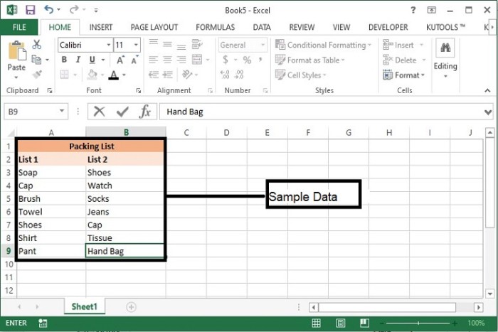
Comparing two columns in Excel and removing matching entries is straightforward using formulas and filters. COMPARE.EDU.VN provides detailed guides and tools to make this process even easier, helping you efficiently manage your data. This article explores methods for identifying and deleting duplicates, ensuring data accuracy and streamlining your spreadsheets. Looking for ways to dedupe data? Explore advanced filtering techniques and data manipulation.

1. Why Compare Columns and Delete Matches in Excel?

Why should you learn How To Compare Two Columns And Delete Matches In Excel? Imagine you are managing a large customer database or a product inventory. Duplicate entries can lead to errors, wasted resources, and inaccurate reports. Comparing columns and removing matches helps you:

• Ensure Data Accuracy: Eliminating duplicates ensures that your data reflects the true state of affairs, whether it’s customer lists or inventory counts.
• Improve Efficiency: Clean data leads to faster processing and analysis. No more sifting through redundant information.
• Reduce Errors: By removing duplicates, you reduce the risk of making incorrect decisions based on flawed data.
• Optimize Resources: For instance, in marketing, you avoid sending the same promotional material to the same customer twice.

1.1 Real-World Scenarios

Consider these scenarios where comparing columns and deleting matches can be a game-changer:

• Customer Relationship Management (CRM):
  • Challenge: Duplicate customer entries can clutter your CRM, leading to confusion and inefficient communication.
  • Solution: Regularly compare email or phone number columns and delete matches to maintain a clean and accurate customer list.
• Inventory Management:
  • Challenge: Duplicate product entries can skew inventory counts and lead to ordering errors.
  • Solution: Compare product ID or name columns to eliminate redundant entries and ensure accurate stock levels.
• Event Planning:
  • Challenge: Duplicate registrations can cause confusion and affect logistics.
  • Solution: Compare registration columns (e.g., email addresses) to remove duplicates and get an accurate attendee count.
• Academic Research:
  • Challenge: In research data, duplicate entries can bias results and affect the validity of findings.
  • Solution: Compare relevant columns (e.g., participant IDs) to eliminate duplicates and ensure data integrity.

1.2 Common Challenges

Before diving into the solutions, it’s important to acknowledge some common challenges users face:

• Large Datasets: Manually comparing thousands of rows is impractical and prone to error.
• Data Inconsistencies: Slight variations in data entry (e.g., “John Smith” vs. “John S.”) can make it difficult to identify duplicates.
• Complex Criteria: Sometimes, you need to compare based on multiple criteria (e.g., name and address) to accurately identify duplicates.

2. Understanding the Basics of Excel

Before we get into the specifics, let’s cover some essential Excel features that you’ll use frequently.

2.1 Essential Excel Functions

These functions are the building blocks for comparing columns:

• MATCH Function: The MATCH function searches for a specified item in a range of cells and returns the relative position of that item in the range.
  • Syntax: MATCH(lookup_value, lookup_array, [match_type])
  • Example: MATCH("apple", A1:A10, 0) finds “apple” in the range A1 to A10 and returns its position. The 0 signifies an exact match.
• ISERROR Function: The ISERROR function checks whether a cell contains an error value (#N/A, #VALUE!, #REF!, #DIV/0!, #NUM!, #NAME?, or #NULL!). It returns TRUE if the cell contains an error and FALSE otherwise.
  • Syntax: ISERROR(value)
  • Example: ISERROR(A1) checks if cell A1 contains an error.
• IF Function: The IF function checks whether a condition is met and returns one value if TRUE and another value if FALSE.
  • Syntax: IF(logical_test, value_if_true, value_if_false)
  • Example: IF(A1>10, "Over 10", "10 or Less") returns “Over 10” if the value in A1 is greater than 10, and “10 or Less” otherwise.
• COUNTIF Function: The COUNTIF function counts the number of cells within a range that meet a given criteria.
  • Syntax: COUNTIF(range, criteria)
  • Example: COUNTIF(A1:A10, "apple") counts the number of cells in the range A1 to A10 that contain “apple”.

2.2 Using Filters in Excel

Filters allow you to display only the rows that meet certain criteria, making it easier to manage and manipulate data.

• How to Apply a Filter:
  1. Select the header row of your data.
  2. Go to the “Data” tab on the Excel ribbon.
  3. Click the “Filter” button. Dropdown arrows will appear in each header cell.
• Filtering Data:
  1. Click the dropdown arrow in the column you want to filter.
  2. Use the checkboxes to select the values you want to display.
  3. Click “OK” to apply the filter.

2.3 Conditional Formatting

Conditional formatting allows you to automatically apply formatting (e.g., colors, icons) to cells based on specific criteria. This can be incredibly useful for highlighting duplicates.

• How to Apply Conditional Formatting to Highlight Duplicates:
  1. Select the range of cells you want to check for duplicates.
  2. Go to the “Home” tab on the Excel ribbon.
  3. Click “Conditional Formatting” in the “Styles” group.
  4. Select “Highlight Cells Rules” and then “Duplicate Values.”
  5. Choose the formatting style you want to use to highlight duplicates (e.g., light red fill with dark red text).
  6. Click “OK.”

3. Method 1: Using Formulas to Identify and Delete Matches

This method involves using a combination of Excel formulas to flag duplicate entries.

3.1 Step-by-Step Guide

1. Set Up Your Data:

   • Assume you have two columns, A and B, with your data.
   • Add a header row to label your columns (e.g., “Column A” and “Column B”).
     

2. Use the MATCH and ISERROR Functions:

   • In column C, starting from C2, enter the following formula:

     =IF(ISERROR(MATCH(A2,B:B,0)),"Unique","Duplicate")

   • This formula checks if the value in cell A2 exists in column B. If it does, it marks it as “Duplicate”; otherwise, it marks it as “Unique.”

3. Drag the Formula Down:

   • Click and drag the bottom-right corner of cell C2 down to apply the formula to all rows in your data.
     

4. Filter for Duplicates:

   • Select the header row (including the new column C).
   • Go to the “Data” tab and click “Filter.”
   • Click the dropdown arrow in column C and select “Duplicate.” This will display only the rows where the value in column A is also found in column B.
     

5. Delete the Matched Rows:

   • With the filtered view, select all the visible rows (the duplicate rows).
   • Right-click on the selected rows and choose “Delete Row.”
     

6. Remove the Filter:

   • Go to the “Data” tab and click “Filter” again to remove the filter and display all rows.
   • Column A now contains only unique values that were not found in column B.

3.2 Formula Explanation

Let’s break down the formula =IF(ISERROR(MATCH(A2,B:B,0)),"Unique","Duplicate"):

• MATCH(A2,B:B,0): This part of the formula searches for the value in cell A2 within the entire column B. The 0 specifies that you want an exact match. If a match is found, the MATCH function returns the row number where the match occurs. If no match is found, it returns an error (#N/A).
• ISERROR(...): This function checks if the result of the MATCH function is an error. If MATCH returns an error (meaning no match was found), ISERROR returns TRUE. Otherwise, it returns FALSE.
• IF(ISERROR(...), "Unique", "Duplicate"): This is the main part of the formula. It checks the result of the ISERROR function. If ISERROR returns TRUE (meaning no match was found), the IF function returns “Unique.” If ISERROR returns FALSE (meaning a match was found), the IF function returns “Duplicate.”

3.3 Pros and Cons

• Pros:
  • Clear Logic: The formulas are relatively straightforward and easy to understand.
  • Non-Destructive: The original data remains intact until you choose to delete the rows.
• Cons:
  • Manual Deletion: Requires manual filtering and deletion of rows.
  • Complexity: Can be cumbersome for users unfamiliar with Excel formulas.

4. Method 2: Using COUNTIF Function for Conditional Deletion

The COUNTIF function provides a more direct way to identify duplicates, which can be used for conditional deletion.

4.1 Step-by-Step Guide

1. Set Up Your Data:

   • As before, assume you have two columns, A and B, with your data.
   • Add a header row to label your columns.

2. Use the COUNTIF Function:

   • In column C, starting from C2, enter the following formula:

     =COUNTIF(B:B,A2)

   • This formula counts how many times the value in cell A2 appears in column B.

3. Drag the Formula Down:

   • Click and drag the bottom-right corner of cell C2 down to apply the formula to all rows in your data.

4. Filter for Values Greater Than 0:

   • Select the header row (including the new column C).
   • Go to the “Data” tab and click “Filter.”
   • Click the dropdown arrow in column C.
   • Choose “Number Filters” and then “Greater Than.”
   • Enter 0 in the dialog box and click “OK.” This will display only the rows where the value in column A appears in column B at least once.
     

5. Delete the Matched Rows:

   • With the filtered view, select all the visible rows (the duplicate rows).
   • Right-click on the selected rows and choose “Delete Row.”

6. Remove the Filter:

   • Go to the “Data” tab and click “Filter” again to remove the filter and display all rows.

4.2 Formula Explanation

The formula =COUNTIF(B:B,A2) is more straightforward:

• COUNTIF(B:B,A2): This counts the number of times the value in cell A2 appears in column B. If the value appears at least once, it means it’s a duplicate.

4.3 Pros and Cons

• Pros:
  • Simplicity: Easier to understand and implement than the MATCH and ISERROR combination.
  • Direct Indication: Directly shows how many times the value appears in the other column.
• Cons:
  • Still Requires Manual Deletion: Like the previous method, it requires manual filtering and deletion.

5. Method 3: Using Advanced Filter

Excel’s Advanced Filter offers a powerful way to filter unique records directly, which can be used to remove duplicates.

5.1 Step-by-Step Guide

1. Copy Data:

   • Copy the data from column A to a new column, say column D. This ensures you’re working with a copy and don’t modify your original data.

2. Select Data Range:

   • Select the range of cells containing the data you want to filter (e.g., D1:D10).

3. Open Advanced Filter:

   • Go to the “Data” tab and click “Advanced” in the “Sort & Filter” group.

4. Configure Advanced Filter:

   • In the “Advanced Filter” dialog box:
     • Choose “Copy to another location.”
     • Set the “List range” to the range of cells containing your data (e.g., $D$1:$D$10).
     • Leave the “Criteria range” blank.
     • Check the “Unique records only” box.
     • Set the “Copy to” range to a new location (e.g., $E$1).
     • Click “OK.”
       

5. Check Results:

   • Excel will copy the unique values from column D to column E, effectively removing any duplicates.
   • You can then delete column A if desired, or use the unique values in column E for further analysis.

5.2 Pros and Cons

• Pros:
  • Directly Extracts Unique Values: Simplifies the process of getting unique values without complex formulas.
  • No Manual Deletion: Automatically extracts unique records, eliminating the need for manual deletion.
• Cons:
  • Removes Duplicates Entirely: This method might not be suitable if you need to compare and conditionally delete based on matches with another column.

6. Method 4: Power Query for Advanced Data Cleansing

Power Query is an Excel tool for data transformation and cleansing. It offers advanced features for comparing columns and removing matches.

6.1 Step-by-Step Guide

1. Load Data into Power Query:

   • Select your data range (including headers).
   • Go to the “Data” tab and click “From Table/Range.” This opens the Power Query Editor.
     

2. Create a Duplicate Column:

   • In the Power Query Editor, select the column you want to check for duplicates (e.g., “Column A”).
   • Go to “Add Column” tab and click “Duplicate Column.”

3. Merge Columns:

   • Select the duplicate column and column B.
   • Go to “Transform” tab and click “Merge Columns.”
   • Choose a separator (e.g., “None”) and name the new column (e.g., “Combined”).

4. Add Conditional Column:

   • Go to “Add Column” tab and click “Conditional Column.”
   • Set up a rule: If “Combined” equals [Column A], then “Unique,” else “Duplicate.”

5. Filter for Unique Values:

   • Click the dropdown arrow in the new conditional column and select “Unique.”

6. Remove Unnecessary Columns:

   • Select the columns you no longer need (e.g., the original columns A and B, and the “Combined” column).
   • Right-click and choose “Remove Columns.”

7. Load Data Back to Excel:

   • Go to “Home” tab and click “Close & Load” to load the transformed data back into an Excel sheet.

6.2 Pros and Cons

• Pros:
  • Advanced Transformation Capabilities: Power Query offers a wide range of data transformation tools.
  • Automation: The steps can be saved and repeated for future data updates.
• Cons:
  • Steeper Learning Curve: Power Query has a more complex interface compared to basic Excel features.

7. Troubleshooting Common Issues

When comparing columns and deleting matches, you might encounter some common issues. Here’s how to troubleshoot them.

7.1 Data Type Mismatches

• Problem: Excel might not recognize duplicates if the data types are different (e.g., a number formatted as text).
• Solution:
  • Ensure both columns have the same data type.
  • Select the columns and go to the “Home” tab.
  • Use the dropdown menu in the “Number” group to format the columns as “General,” “Number,” or “Text,” as appropriate.
  • For numbers formatted as text, you can also use the VALUE function to convert them to numbers: =VALUE(A1).

7.2 Inconsistent Data Entry

• Problem: Slight variations in data entry (e.g., “John Smith” vs. “John S.”) can prevent Excel from identifying duplicates.
• Solution:
  • Use the TRIM function to remove extra spaces: =TRIM(A1).
  • Use the CLEAN function to remove non-printable characters: =CLEAN(A1).
  • For more complex inconsistencies, consider using the SUBSTITUTE function to replace specific text: =SUBSTITUTE(A1, "S.", "Smith").

7.3 Formula Errors

• Problem: Errors in your formulas can lead to incorrect results.
• Solution:
  • Double-check the syntax of your formulas.
  • Use Excel’s “Evaluate Formula” tool (in the “Formulas” tab) to step through the formula and identify the source of the error.
  • Ensure that cell references are correct and that you are using absolute references ($) where necessary.

7.4 Performance Issues with Large Datasets

• Problem: Processing large datasets can slow down Excel.
• Solution:
  • Use Excel tables for better performance.
  • Disable automatic calculations while performing complex operations:
    • Go to “Formulas” tab, click “Calculation Options,” and select “Manual.”
    • Remember to switch back to “Automatic” when you’re done.
  • Consider using Power Query, which is designed to handle large datasets more efficiently.

8. Best Practices for Data Management in Excel

To ensure accurate and efficient data management, follow these best practices.

8.1 Data Validation

• What it is: Data validation helps prevent incorrect data entry by setting rules for what can be entered in a cell.
• How to use it:
  • Select the cells where you want to apply data validation.
  • Go to the “Data” tab and click “Data Validation.”
  • Set the criteria for allowed values (e.g., whole numbers, dates within a certain range, or a list of predefined values).
• Example: Restricting entries in a “Country” column to a predefined list of countries.

8.2 Consistent Formatting

• Why it matters: Consistent formatting ensures that data is uniform and easier to analyze.
• How to achieve it:
  • Use Excel’s formatting tools to apply consistent styles to your data.
  • Use the “Format Painter” to copy formatting from one cell to another.
  • Create and use Excel tables, which automatically apply consistent formatting.

8.3 Regular Data Cleansing

• Why it matters: Regular data cleansing helps maintain data accuracy and prevents the accumulation of errors.
• How to do it:
  • Schedule regular data cleansing tasks.
  • Use the methods described in this article to identify and remove duplicates.
  • Correct any data entry errors.
  • Update outdated information.

8.4 Backups

• Why it matters: Backups protect your data from loss due to hardware failures, software errors, or accidental deletion.
• How to do it:
  • Regularly save your Excel files to a secure location.
  • Consider using cloud-based storage solutions like OneDrive or Google Drive, which automatically back up your files.
  • Create backup copies of your files before performing major data manipulations.

9. Advanced Techniques and Tips

For those looking to take their Excel skills to the next level, here are some advanced techniques and tips.

9.1 Using VBA for Automated Deletion

• What it is: VBA (Visual Basic for Applications) is a programming language that allows you to automate tasks in Excel.

• How to use it:

  • Press Alt + F11 to open the VBA editor.
  • Insert a new module (Insert > Module).
  • Write VBA code to compare columns and delete matches automatically.

• Example Code:

  Sub DeleteDuplicates()
      Dim i As Long, LastRow As Long
      LastRow = Cells(Rows.Count, "A").End(xlUp).Row 'Find the last row in Column A
  
      Application.ScreenUpdating = False
  
      For i = LastRow To 2 Step -1 'Loop through each row from bottom to top
          If WorksheetFunction.CountIf(Range("B:B"), Cells(i, "A").Value) > 0 Then
              Rows(i).Delete
          End If
      Next i
  
      Application.ScreenUpdating = True
  End Sub

• Explanation: This VBA code loops through each row in column A and checks if the value exists in column B. If it does, the row is deleted.

• Caution: VBA code can modify your data, so always test it on a backup copy first.

9.2 Combining Multiple Criteria for Identifying Duplicates

• Challenge: Identifying duplicates based on multiple criteria (e.g., name and address).
• Solution:
  • Create a helper column that concatenates the relevant columns: =A2&B2&C2.
  • Use the methods described earlier (e.g., COUNTIF, conditional formatting) on the helper column to identify duplicates based on the combined criteria.

9.3 Using Array Formulas for Complex Comparisons

• What it is: Array formulas allow you to perform calculations on multiple values at once.
• How to use it:
  • Enter the formula and press Ctrl + Shift + Enter to create an array formula.
• Example: To compare two columns and return an array of TRUE or FALSE values indicating whether each row is a duplicate:

  =A1:A10=TRANSPOSE(B1:B10)

• Caution: Array formulas can be computationally intensive, especially on large datasets.

10. Conclusion: Making Data Management Easier with COMPARE.EDU.VN

Managing data in Excel can be complex, but with the right techniques, you can efficiently compare columns and delete matches to ensure data accuracy. Whether you choose to use formulas, filters, Power Query, or VBA, the key is to understand the strengths and limitations of each method and apply them appropriately.

Remember, accurate data management not only saves time but also leads to better decision-making and improved efficiency. For more detailed guides, tools, and resources, visit COMPARE.EDU.VN, your go-to destination for mastering Excel and other essential software skills.

10.1 Your Next Steps

Ready to take control of your data? Here’s how COMPARE.EDU.VN can help:

• Explore Our Guides: Dive into our comprehensive guides on Excel, data management, and more.
• Use Our Tools: Take advantage of our free Excel templates and tools to streamline your data management tasks.
• Join Our Community: Connect with other Excel users and experts to share tips and tricks.

10.2 Contact Us

Have questions or need further assistance? Contact us at:

• Address: 333 Comparison Plaza, Choice City, CA 90210, United States
• WhatsApp: +1 (626) 555-9090
• Website: COMPARE.EDU.VN

Start improving your data management skills today with compare.edu.vn.

FAQ: Comparing Columns in Excel

1. How can I compare two columns in Excel to find matching values?

You can use the MATCH function in combination with the ISERROR and IF functions. The formula would be: =IF(ISERROR(MATCH(A2,B:B,0)),"Unique","Duplicate"). This formula checks if the value in cell A2 exists in column B and returns “Duplicate” if it does, and “Unique” if it doesn’t.

2. What is the best way to delete duplicate rows after comparing two columns?

After identifying duplicate rows using a formula like the one above, you can filter the column with the formula for “Duplicate” and then delete the visible rows. Alternatively, you can use Power Query to filter and remove duplicates more efficiently.

3. Can I compare two columns and highlight the matching values instead of deleting them?

Yes, you can use conditional formatting. Select the range of cells you want to check, go to “Home” > “Conditional Formatting” > “Highlight Cells Rules” > “Duplicate Values,” and choose a formatting style to highlight the matching values.

4. How do I compare two columns with different data types?

Ensure both columns have the same data type by formatting them as “General,” “Number,” or “Text” as appropriate. You can also use the VALUE function to convert numbers formatted as text to numbers: =VALUE(A1).

5. What if there are slight variations in data entry, like “John Smith” vs. “John S.”?

Use the TRIM function to remove extra spaces and the CLEAN function to remove non-printable characters. For more complex inconsistencies, use the SUBSTITUTE function to replace specific text: =SUBSTITUTE(A1, "S.", "Smith").

6. How can I compare two columns based on multiple criteria?

Create a helper column that concatenates the relevant columns: =A2&B2&C2. Then, use the methods described earlier (e.g., COUNTIF, conditional formatting) on the helper column to identify duplicates based on the combined criteria.

7. Is it possible to automate the process of comparing and deleting duplicates in Excel?

Yes, you can use VBA (Visual Basic for Applications) to automate the process. Write VBA code to loop through each row, compare values, and delete duplicates automatically. Always test the code on a backup copy first.

8. What is Power Query, and how can it help with comparing columns?

Power Query is an Excel tool for data transformation and cleansing. It offers advanced features for comparing columns, merging data, and filtering unique records. It can handle large datasets more efficiently than basic Excel features.

9. How do I use the COUNTIF function to compare two columns?

In column C, starting from C2, enter the formula =COUNTIF(B:B,A2). This formula counts how many times the value in cell A2 appears in column B. Filter for values greater than 0 to identify duplicates.

10. What are some best practices for managing data in Excel?

Use data validation to prevent incorrect data entry, maintain consistent formatting, perform regular data cleansing, and create backups of your files. These practices help ensure data accuracy and prevent data loss.