How to compare two columns in Excel? Comparing two columns in Excel is crucial for data analysis, validation, and ensuring data integrity, and COMPARE.EDU.VN provides expert guidance on these techniques. Using Excel formulas, conditional formatting, and lookup functions enables efficient identification of matches, differences, and duplicates in datasets. Enhance your data management skills with COMPARE.EDU.VN, which offers resources on data comparison tools, data validation methods, and data analysis strategies.
1. Why is Comparing Two Columns in Excel Useful?
Comparing two columns in Excel is a fundamental task with numerous applications. Excel’s versatility in data storage and manipulation makes it an essential tool for data analysts and decision-makers. By comparing two columns, you can identify matching entries, find discrepancies, and ensure data consistency across your spreadsheets. This process is vital for tasks such as validating data entry, identifying duplicates, and comparing datasets from different sources. A data analyst uses these comparisons to determine whether a cell contains data. Excel displays it as TRUE/FALSE, Match/Not Match, or user-defined messages, greatly aiding decision-making processes.
2. What Methods Can Be Used to Compare Two Columns in Excel?
There are several methods to compare two columns in Excel, each with its own advantages depending on the specific comparison requirements. These methods include:
- Highlighting unique or duplicate values using functions.
- Displaying unique or duplicate cells using conditional formatting or formulas.
- Performing row-by-row comparisons using formulas.
- Using LOOKUP functions to find matching values.
These techniques allow for flexibility in comparing data based on the desired outcome and the structure of the data.
3. How Do You Compare Two Columns Using the Equals Operator?
Comparing two columns using the equals operator is a straightforward method for identifying matching data on a row-by-row basis.
Here’s how to do it:
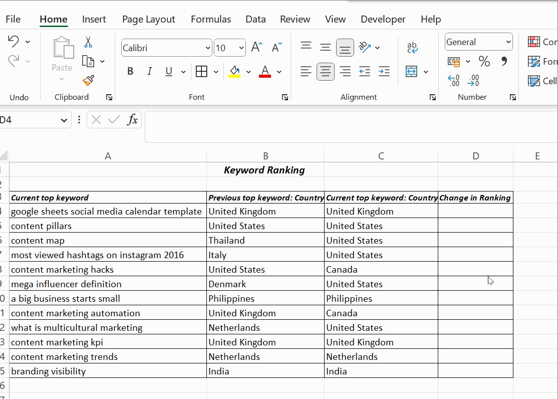
- Enter the Formula: In an empty column (e.g., column D), enter the formula
=B4=C4in cell D4, assuming your data starts in row 4 of columns B and C. - Apply the Formula: Drag the formula down to apply it to the rest of the rows in your dataset.
- Interpret the Results: The formula returns TRUE if the values in columns B and C match for that row and FALSE if they differ.
This method is quick and easy for basic comparisons.
4. How Do You Compare Two Columns Using the IF Condition?
The IF condition allows you to display custom messages based on whether the values in two columns match. Here are a few ways to use the IF condition:
4.1. Displaying “Yes” or Empty
You can use the formula =IF(B4=C4,"Yes"," ") to display “Yes” for matching rows and leave the cell empty for non-matching rows. This method is useful for quickly identifying matching entries without cluttering the spreadsheet with “No” or “False” values.
4.2. Displaying “Yes” or “No”
To display “Yes” for matching rows and “No” for non-matching rows, use the formula =IF(B4=C4,"Yes","No"). This provides a clear indication of whether each row matches or not.
4.3. Comparing for Differences
To compare two columns for differences, replace the equals sign with the not-equal-to sign (<>). The formula =IF(B4<>C4,"Not a Match","Match") will display “Not a Match” for rows where the values differ and “Match” for rows where they are the same.
5. How Can the EXACT() Function Be Used for Case-Sensitive Comparisons?
The EXACT() function ensures that comparisons are case-sensitive, which is crucial when differentiating between text entries that may only differ in capitalization. The syntax for the EXACT() function is =EXACT(text1,text2).
To use EXACT() in combination with the IF condition, use the formula =IF(EXACT(B4,C4), "Match", "Mismatched"). This formula returns “Match” only if the text in both cells is identical, including capitalization, and “Mismatched” otherwise.
This is especially useful for ensuring data accuracy when capitalization matters.
6. How Do You Compare Two Columns in Excel Using Conditional Formatting?
Conditional formatting is a powerful tool for visually highlighting matching or unique values in two columns. Here’s how to use it:
- Select the Columns: Select the columns you want to compare.
- Open Conditional Formatting: Go to Home → Styles → Conditional Formatting → Highlight Cell Rules.
- Choose Duplicate Values: Select Duplicate Values to highlight values that appear in both columns.
- Customize Formatting: Choose the formatting style (e.g., fill color, text color) you want to apply to the duplicate values.
- Highlight Unique Values: Alternatively, select Unique Values to highlight values that appear only in one of the columns.
This method allows you to quickly visualize the similarities and differences between the two columns without using additional formulas.
7. How Do You Use the LOOKUP Function to Compare Two Columns?
The LOOKUP function can be used to compare two columns and return corresponding values based on matches. There are several types of LOOKUP functions, including HLOOKUP, VLOOKUP, and XLOOKUP. Here’s an example using VLOOKUP:
7.1. Example Using VLOOKUP
Suppose you have two columns: Column A contains a list of keywords, and Column B contains parent keywords. To find the matching parent keyword for each keyword in Column A, you can use the following formula in Column C:
=VLOOKUP(A4, $B$4:$B$15, 1, 0)
This formula does the following:
- VLOOKUP(A4, …): Looks up the value in cell A4.
- VLOOKUP(A4, $B$4:$B$15, …): Searches for the value in the range B4 to B15. The
$symbols create an absolute reference, ensuring the range doesn’t change when you drag the formula down. - VLOOKUP(A4, $B$4:$B$15, 1, …): Returns the value from the first column (in this case, the same column being searched).
- VLOOKUP(A4, $B$4:$B$15, 1, 0): Specifies that you want an exact match.
This formula will return the matching parent keyword from Column B for each keyword in Column A.
8. How Can You Compare Three or More Columns in Excel?
Comparing three or more columns in Excel requires using more complex formulas that combine IF and AND statements. Here’s how:
8.1. Finding Matches in All Columns
To find matches in all cells across three or more columns, use the following formula:
=IF(AND(A2=B2, A2=C2), "Full match", "")
This formula checks if the values in cells A2, B2, and C2 are all the same. If they are, it returns “Full match”; otherwise, it returns an empty string.
8.2. Finding Matches in Any Two Columns
To find matches in any two cells in the same row, use the following formula:
=IF(OR(A2=B2, B2=C2, A2=C2), "Match", "")
This formula checks if any two cells among A2, B2, and C2 have the same value. If any match is found, it returns “Match”; otherwise, it returns an empty string.
9. How Do You Compare Two Columns and Highlight Row Differences?
To compare two columns and highlight the row differences, you can use a combination of conditional formatting and formulas.
9.1. Using the “Go To Special” Feature
- Select the Columns: Select the two columns you want to compare.
- Open “Go To Special”: Go to Home → Find & Select → Go To Special.
- Choose “Row Differences”: Select Row Differences and click OK.
This will highlight the cells that differ between the two columns. The matching data cells across the columns’ rows are white, and unmatched cells appear in gray.
9.2. Using Conditional Formatting with a Formula
- Select the Data Range: Select the range of cells you want to apply the formatting to.
- Open Conditional Formatting: Go to Home → Styles → Conditional Formatting → New Rule.
- Use a Formula: Select Use a formula to determine which cells to format.
- Enter the Formula: Enter the formula
=A2<>B2, where A2 and B2 are the first cells in your data range. - Format the Cells: Click Format and choose the formatting style you want to apply to the differing cells.
- Apply the Rule: Click OK to apply the rule.
This will highlight the cells in Column A that are different from the corresponding cells in Column B.
10. How Can COMPARE.EDU.VN Help with Excel Data Comparison?
COMPARE.EDU.VN offers comprehensive resources and guidance on mastering Excel data comparison techniques. Whether you’re a student, professional, or data enthusiast, the website provides valuable insights and tools to enhance your data management skills.
COMPARE.EDU.VN helps by:
- Providing detailed tutorials on various Excel functions and formulas for data comparison.
- Offering step-by-step guides on using conditional formatting for visual data analysis.
- Explaining advanced techniques for comparing multiple columns and datasets.
- Offering expert advice on troubleshooting common issues in Excel data comparison.
By leveraging the resources at COMPARE.EDU.VN, users can streamline their data analysis processes, ensure data accuracy, and make informed decisions based on reliable data comparisons.
Excel provides a range of methods for comparing two columns, from simple formulas to advanced conditional formatting and lookup functions. These techniques enable you to identify matches, differences, and duplicates efficiently. For more in-depth tutorials and resources, visit COMPARE.EDU.VN.
Frequently Asked Questions
1. How do you compare two columns in Excel for differences?
To compare two columns in Excel for differences, use the formula =IF(A2<>B2, "Different", "Same"). This formula checks if the values in cells A2 and B2 are different. If they are, it returns “Different”; otherwise, it returns “Same”. You can also use conditional formatting to highlight the different cells.
2. How can I compare two columns and return a value from a third column?
You can use the VLOOKUP function to compare two columns and return a value from a third column. For example, if you want to check if the values in column A exist in column B and return the corresponding value from column C, use the formula =VLOOKUP(A2, B:C, 2, FALSE). This formula searches for the value in A2 within column B and returns the corresponding value from column C.
3. Is there a way to compare two columns and highlight the entire row if there is a match?
Yes, you can use conditional formatting with a formula to highlight the entire row if there is a match. Select the entire data range, then go to Home → Conditional Formatting → New Rule → Use a formula to determine which cells to format. Enter the formula =$A2=$B2 and choose the formatting style you want to apply. This will highlight the entire row if the values in columns A and B match.
4. How do I compare two columns for partial matches?
To compare two columns for partial matches, you can use the SEARCH function combined with the IF function. For example, the formula =IF(ISNUMBER(SEARCH(A2, B2)), "Partial Match", "No Match") checks if the text in cell A2 is found within cell B2. If it is, it returns “Partial Match”; otherwise, it returns “No Match”.
5. Can I compare two columns in different Excel sheets?
Yes, you can compare two columns in different Excel sheets by referencing the sheet name in your formulas. For example, to compare column A in Sheet1 with column A in Sheet2, use the formula =IF(Sheet1!A2=Sheet2!A2, "Match", "No Match") in a third sheet or one of the existing sheets.
6. How do I ignore case when comparing two columns in Excel?
To ignore case when comparing two columns, use the UPPER or LOWER function to convert the text to the same case before comparing. For example, the formula =IF(UPPER(A2)=UPPER(B2), "Match", "No Match") converts the text in both cells to uppercase before comparing them, effectively ignoring case.
7. What is the best way to compare two large columns of data in Excel?
For large datasets, using helper columns with formulas and then filtering or sorting the results is often the most efficient method. Use formulas like =IF(A2=B2, "Match", "No Match") in a helper column, then filter or sort the helper column to quickly identify matches and differences.
8. How do I compare two columns and count the number of matches?
To count the number of matches between two columns, use the SUMPRODUCT function. For example, the formula =SUMPRODUCT(--(A1:A10=B1:B10)) counts the number of rows where the values in column A (A1:A10) are equal to the values in column B (B1:B10).
9. Can I compare two columns and highlight duplicates in both columns?
Yes, you can use conditional formatting to highlight duplicates in both columns. Select both columns, then go to Home → Conditional Formatting → Highlight Cells Rules → Duplicate Values. Choose the formatting style you want to apply, and Excel will highlight the duplicate values in both columns.
10. How do I compare two columns and find the values that are only in one column but not the other?
To find the values that are only in one column but not the other, you can use a combination of COUNTIF and IF functions. In a helper column, use the formula =IF(COUNTIF($B$1:$B$10, A1)=0, "Unique to A", "") to identify values in column A that are not in column B. Similarly, use =IF(COUNTIF($A$1:$A$10, B1)=0, "Unique to B", "") to identify values in column B that are not in column A.
Conclusion
Comparing two columns in Excel is essential for data validation, analysis, and decision-making. Whether using simple formulas, conditional formatting, or advanced functions like VLOOKUP and EXACT, Excel offers a wide range of tools to suit different comparison needs.
For additional resources and in-depth tutorials on mastering Excel, visit COMPARE.EDU.VN.
Need to compare products or services to make a better decision? Visit COMPARE.EDU.VN for comprehensive comparisons and expert insights. Our detailed analyses help you weigh the pros and cons, features, and benefits, ensuring you make the right choice. Make informed decisions with COMPARE.EDU.VN today.
Contact us:
Address: 333 Comparison Plaza, Choice City, CA 90210, United States
WhatsApp: +1 (626) 555-9090
Website: compare.edu.vn