Comparing data in two columns in Excel is crucial for data analysis and decision-making, and COMPARE.EDU.VN offers comprehensive guides to simplify this process. By utilizing functions like IF, EXACT, and VLOOKUP, along with conditional formatting, you can efficiently identify matching, mismatching, unique, or duplicate values. Explore advanced comparison techniques and data matching strategies to enhance your spreadsheet analysis skills.
1. Why Is Comparing Two Columns in Excel Useful?
Excel’s data comparison features are essential for data analysts who need to make informed decisions based on data, allowing them to quickly identify whether a cell contains specific information across the same or different spreadsheets. Instead of manual, time-consuming comparisons, Excel provides tools that display results as TRUE/FALSE, Match/Not Match, or other user-defined messages, thereby increasing efficiency and accuracy. Comparing data effectively can help reveal data patterns, detect errors, and confirm data integrity.
2. What Methods Can Be Used to Compare Two Columns in Excel?
Excel offers multiple methods to compare columns, each serving different comparison needs. You can use functions to highlight unique or duplicate values, apply conditional formatting to display unique or duplicate cells, conduct row-by-row comparisons, or leverage LOOKUP formulas for more complex comparisons. Each technique provides a unique way to identify and analyze data differences and similarities within your spreadsheets.
3. How Do You Compare Two Columns Using the Equals Operator in Excel?
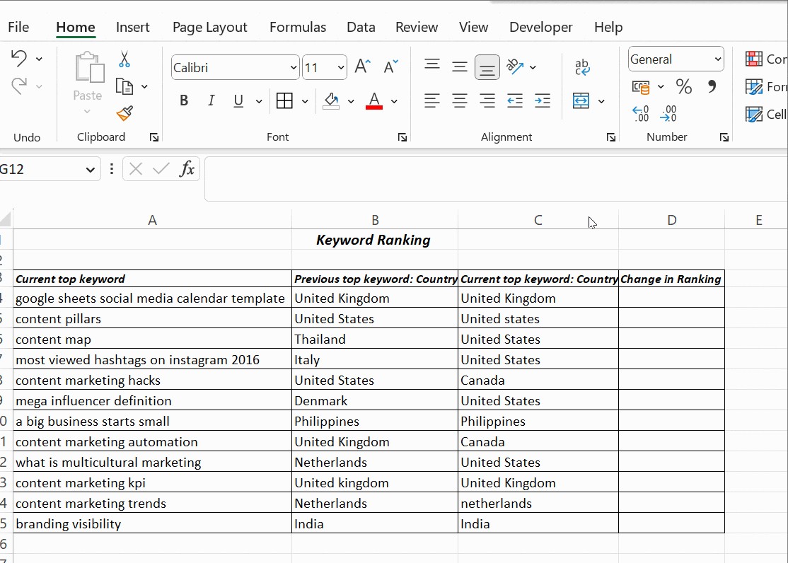
Comparing two columns row by row and displaying the results as “Match” or “Not Match” can be done using the equals operator (=). The formula =column1=column2 returns “TRUE” if the values in the compared columns are the same and “FALSE” otherwise. This straightforward method provides a quick visual comparison of data across rows.
For example, if you have data in columns B and C, you can enter the formula =B4=C4 in cell D4 and drag it down to apply it to all rows. This will show TRUE or FALSE based on whether the values in columns B and C match.
4. How Can the IF Condition Be Used to Compare Two Columns in Excel?
The IF condition in Excel allows you to customize the comparison results, such as displaying “Yes” for matching values and leaving other cells blank. The formula =IF(B4=C4,"Yes","") returns “Yes” for rows with matching values and an empty string for non-matching rows. This is a flexible way to highlight matches and easily spot differences.
You can also use the IF condition to identify mismatching values by including an additional argument when the IF condition proves false. The formula =IF(B4=C4,"Yes","No") returns “Yes” for matching values and “No” for mismatching values, providing a clear distinction between the two.
To specifically compare two columns for differences, you can replace the equals sign with the non-equality sign (<>). The formula =IF(A2<>B2,"Match","Not a Match") will return “Match” if the values in columns A and B are different, and “Not a Match” if they are the same.
5. How Does the EXACT() Function Enhance Column Comparisons in Excel?
The EXACT() function enhances column comparisons by ensuring that the capitalization of text strings matches exactly. Unlike the standard equals operator, EXACT() is case-sensitive, making it ideal for situations where capitalization is crucial. The syntax is =EXACT(text1,text2), and it returns TRUE only if the text strings are identical, including capitalization.
To use EXACT() with an IF condition, you can use the formula =IF(EXACT(B4,C4), "Match", "Mismatched"). This formula returns “Match” only if the values in columns B and C are identical, including capitalization, and “Mismatched” otherwise.
6. How Can Conditional Formatting Be Used to Compare Columns in Excel?
Conditional formatting in Excel provides a visual way to highlight duplicate or unique values in columns without needing a third column for results. By selecting Home → Conditional Formatting → Highlight Cells Rules → Duplicate Values, you can apply formatting conditions such as color fills, text color changes, or cell borders to highlight matching or unique data. This method is particularly useful for quickly identifying patterns in large datasets.
To highlight data present in both columns, select the columns, choose “Duplicate” from the conditional formatting options, and select a formatting style. This will highlight all cells containing values found in both columns. Alternatively, you can select “Unique” to highlight cells with data that is not repeated in the selected columns.
If you want to clear the formatting, go to Conditional Formatting → Clear Rules → Clear Rules from Selected Cells. This will remove any conditional formatting applied to the selected cells.
7. How Do Lookup Functions Facilitate Column Comparisons in Excel?
Lookup functions like VLOOKUP are useful for comparing two columns and finding related information. VLOOKUP searches for a value in one column and returns a corresponding value from another column. This function is particularly useful when you need to find matches based on specific criteria.
For example, if column A contains a list of keywords and column B contains parent keywords, you can use VLOOKUP to find the parent keyword for each keyword in column A. The formula might look like this: =VLOOKUP(A4, $B$4:$B$15, 1, 0).
In this formula:
A4is the lookup value (the keyword you are searching for).$B$4:$B$15is the range where the parent keywords are located (locked using absolute reference).1indicates that you want to return the value from the first column in the range (the parent keyword).0specifies that you want an exact match.
8. What Are Some Practical Examples of Using Formulas for Data Comparison?
Below are a few practical examples.
8.1. Comparing Email Lists
Imagine you have two lists of email addresses in columns A and B. You want to identify which email addresses are present in both lists. Using the formula =IF(COUNTIF(B:B, A1)>0, "Yes", "No") in column C, you can check if each email in column A exists in column B. If the result is “Yes,” the email is present in both lists.
8.2. Verifying Product IDs
Suppose you have a list of product IDs in column A and a list of valid IDs in column B. You want to ensure that all IDs in column A are valid. Using the formula =IF(ISNUMBER(MATCH(A1, B:B, 0)), "Valid", "Invalid") in column C, you can check if each product ID in column A exists in column B. If the result is “Valid,” the ID is correct.
8.3. Identifying Missing Data
If you have a list of dates in column A and another list in column B, you can find which dates are missing from column B using the formula =IF(ISNA(MATCH(A1, B:B, 0)), "Missing", "") in column C. This formula checks if each date in column A exists in column B and flags the missing dates.
9. How Do You Compare Three or More Columns in Excel?
To compare three or more columns in Excel, you can use a combination of IF() and AND() functions to find matches across all columns, or IF() and OR() functions to find matches in any two columns. For example, the formula =IF(AND(A2=B2, A2=C2), "Full Match", "") returns “Full Match” only if the values in columns A, B, and C are identical. The formula =IF(OR(A2=B2, B2=C2, A2=C2), "Match", "") returns “Match” if any two columns have matching values.
10. What Are Some Common Mistakes to Avoid When Comparing Columns?
When comparing columns in Excel, it’s important to avoid common mistakes such as overlooking case sensitivity, ignoring hidden characters, and not using absolute references properly. Case sensitivity can be addressed using the EXACT() function, while hidden characters can be removed using the TRIM() function. Ensuring that you use absolute references (e.g., $B$4:$B$15) when necessary will prevent your formulas from changing unexpectedly as you drag them down.
Conclusion: Streamlining Data Comparison with Excel
Comparing data in two columns in Excel is crucial for data analysis, validation, and decision-making. Whether you need to identify duplicates, find unique entries, or verify data consistency, Excel provides a range of tools and techniques to streamline the process. By mastering functions like IF, EXACT, VLOOKUP, and conditional formatting, you can efficiently compare data and gain valuable insights from your spreadsheets. Visit COMPARE.EDU.VN for more in-depth tutorials and advanced strategies to enhance your Excel skills.
Ready to take your Excel skills to the next level? At COMPARE.EDU.VN, we provide comprehensive guides and resources to help you master data comparison techniques and make informed decisions. Whether you’re analyzing financial data, comparing product lists, or verifying customer information, our expert insights will help you streamline your workflow and improve your accuracy.
Visit COMPARE.EDU.VN today and explore our extensive collection of Excel tutorials, tips, and tricks. Let us help you unlock the full potential of Excel and become a data comparison expert.
Address: 333 Comparison Plaza, Choice City, CA 90210, United States
WhatsApp: +1 (626) 555-9090
Website: compare.edu.vn