Comparing data in Excel is crucial for data analysis and decision-making, and at COMPARE.EDU.VN, we provide comprehensive guides to simplify this process. Discover effective methods to compare data, identify differences, and ensure data accuracy, all while leveraging Excel’s powerful features. Let’s explore data comparison techniques, spreadsheet analysis, and data validation.
Table of Contents
- Why Is Comparing Data in Excel Important?
- Different Methods to Compare Data in Excel
- Using the Equals Operator to Compare Two Columns
- Leveraging the IF Condition for Data Comparison
- Employing the EXACT() Function for Case-Sensitive Comparisons
- Conditional Formatting: Highlighting Differences and Duplicates
- Using LOOKUP Functions to Compare Data
- Step-by-Step Guide: Comparing Data in Excel
- FAQ: Common Questions About Comparing Data in Excel
- Conclusion: compare.edu.vn – Your Partner in Data Analysis
1. Why Is Comparing Data in Excel Important?
Comparing data in Excel is an essential skill for anyone working with spreadsheets. It enables you to identify discrepancies, validate data, and derive meaningful insights. Whether you’re a student, professional, or data enthusiast, understanding how to compare data efficiently can significantly enhance your productivity and decision-making.
1.1 Data Validation
Comparing data ensures accuracy. By comparing datasets, you can identify and correct errors, ensuring that your information is reliable. This is especially crucial in fields like finance, where even minor inaccuracies can have significant consequences.
1.2 Identifying Discrepancies
Data comparison helps in spotting inconsistencies between different sources. This is useful when merging datasets or auditing information. Recognizing discrepancies early allows for prompt corrective action.
1.3 Decision Making
Accurate comparisons are essential for informed decision-making. By analyzing data side-by-side, you can make better decisions based on reliable information. This is invaluable for strategic planning and problem-solving.
1.4 Saving Time
Manual data comparison can be time-consuming and error-prone. Excel offers efficient tools to automate this process, saving you valuable time and effort. Automated comparisons reduce the risk of human error and allow you to focus on analysis and interpretation.
1.5 Performance Tracking
Businesses often use Excel to track performance metrics. Comparing current data against historical data helps in identifying trends and evaluating the effectiveness of strategies. This ongoing comparison is crucial for continuous improvement.
2. Different Methods to Compare Data in Excel
Excel provides multiple methods for comparing data, each with its own strengths and use cases. Understanding these methods will allow you to choose the most appropriate technique for your specific needs.
2.1 Using the Equals Operator
The equals operator (=) is a straightforward way to compare two cells and determine if they contain the same value. This method is simple and effective for basic comparisons.
2.2 IF Condition
The IF condition allows you to perform logical comparisons and return different results based on whether the condition is true or false. This is useful for flagging discrepancies or highlighting matches.
2.3 EXACT() Function
The EXACT() function is case-sensitive, making it ideal for comparing text strings where case matters. This function ensures that comparisons are precise and accurate.
2.4 Conditional Formatting
Conditional formatting allows you to highlight cells based on specific criteria, such as duplicates or unique values. This method provides a visual way to identify patterns and anomalies in your data.
2.5 LOOKUP Functions
LOOKUP functions, like VLOOKUP and XLOOKUP, can be used to compare data across different columns or sheets. These functions are particularly useful for finding matching values in large datasets.
2.6 Using Formulas
Formulas can be created to execute different comparison types. Using formulas, you can compare more than 2 columns. Additionally, you can use formulas to evaluate complex criteria and derive custom comparison results.
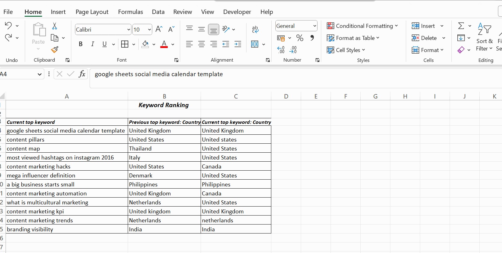
3. Using the Equals Operator to Compare Two Columns
The equals operator (=) is one of the simplest and most direct methods for comparing two columns in Excel. This method is best suited for basic comparisons where you want to know if two cells have the exact same value.
3.1 How to Use the Equals Operator
To use the equals operator, follow these steps:
-
Open your Excel sheet: Launch Microsoft Excel and open the spreadsheet containing the data you want to compare.
-
Select an empty column: Choose a column where you want to display the comparison results. This column should be next to the columns you are comparing.
-
Enter the formula: In the first cell of the empty column, enter the formula
=A1=B1, replacingA1andB1with the first cells you want to compare.- For example, if you want to compare cells
C2andD2, the formula would be=C2=D2.
- For example, if you want to compare cells
-
Drag the formula down: Click on the bottom-right corner of the cell containing the formula (the fill handle) and drag it down to apply the formula to all rows in the column.
-
Review the results: Excel will display
TRUEif the values in the compared cells are the same andFALSEif they are different.
3.2 Example
Let’s say you have two columns, A and B, containing names. You want to compare these columns to see which names match.
| Row | Column A (Name) | Column B (Name) | Column C (Comparison) |
|---|---|---|---|
| 1 | John | John | TRUE |
| 2 | Alice | Alicia | FALSE |
| 3 | Bob | Bob | TRUE |
| 4 | Charlie | Charles | FALSE |

In cell C1, you would enter the formula =A1=B1. After dragging the formula down, column C will show TRUE for rows where the names in column A and column B match, and FALSE where they don’t.
3.3 Advantages
- Simple and easy to use: The equals operator is straightforward and requires no advanced Excel knowledge.
- Real-time results: As you update the data in the compared columns, the comparison results will update automatically.
- Quick identification of matches: You can quickly see which cells have matching values.
3.4 Limitations
- Case-sensitive: The equals operator is case-sensitive. “John” and “john” will be considered different.
- Exact match required: Only provides an exact match comparison. Slight differences, such as extra spaces, will result in a “FALSE” result.
- Limited to exact matches: It cannot identify partial matches or similarities, only exact matches.
- Not suitable for large datasets: For extensive datasets, manually reviewing
TRUEandFALSEvalues can be time-consuming.
4. Leveraging the IF Condition for Data Comparison
The IF condition in Excel allows you to perform logical comparisons and return different results based on whether the condition is true or false. This method is more versatile than the equals operator and can be customized to provide more informative results.
4.1 How to Use the IF Condition
To use the IF condition, follow these steps:
-
Open your Excel sheet: Launch Microsoft Excel and open the spreadsheet containing the data you want to compare.
-
Select an empty column: Choose a column where you want to display the comparison results.
-
Enter the formula: In the first cell of the empty column, enter the formula
=IF(A1=B1, "Match", "Not Match"), replacingA1andB1with the first cells you want to compare.- This formula checks if the value in cell
A1is equal to the value in cellB1. If it is, the formula returns “Match”; otherwise, it returns “Not Match”.
- This formula checks if the value in cell
-
Drag the formula down: Click on the bottom-right corner of the cell containing the formula (the fill handle) and drag it down to apply the formula to all rows in the column.
-
Review the results: Excel will display “Match” for rows where the values in the compared columns are the same and “Not Match” where they are different.
4.2 Example
Continuing with the example of comparing names in columns A and B:
| Row | Column A (Name) | Column B (Name) | Column C (Comparison) |
|---|---|---|---|
| 1 | John | John | Match |
| 2 | Alice | Alicia | Not Match |
| 3 | Bob | Bob | Match |
| 4 | Charlie | Charles | Not Match |
In cell C1, you would enter the formula =IF(A1=B1, "Match", "Not Match"). After dragging the formula down, column C will show “Match” for rows where the names in column A and column B match, and “Not Match” where they don’t.
4.3 Customizing the IF Condition
You can customize the IF condition to return different results or perform more complex comparisons. For example, you can use nested IF statements to check for multiple conditions.
- Checking for differences: To check for differences instead of matches, use the
<>operator:=IF(A1<>B1, "Different", "Same"). - Checking for blank cells: To check if either cell is blank, use the
ANDfunction:=IF(AND(A1="", B1=""), "Both Blank", IF(A1=B1, "Match", "Not Match")).
4.4 Advantages
- Customizable results: You can specify the values returned when the condition is true or false.
- Logical comparisons: The IF condition allows you to perform a wide range of logical comparisons, including equality, inequality, and more.
- Easy to understand: The IF condition is relatively easy to understand and use, even for beginners.
4.5 Limitations
- Case-sensitive: Like the equals operator, the IF condition is case-sensitive by default.
- Can become complex: Nested IF statements can become complex and difficult to manage.
- Exact match required: Only provides an exact match comparison.
- Limited to two conditions: Each IF function can evaluate only one condition at a time.
5. Employing the EXACT() Function for Case-Sensitive Comparisons
When comparing text data in Excel, it’s often important to consider case sensitivity. The EXACT() function allows you to compare two text strings and return TRUE only if they are exactly the same, including case.
5.1 How to Use the EXACT() Function
To use the EXACT() function, follow these steps:
- Open your Excel sheet: Launch Microsoft Excel and open the spreadsheet containing the data you want to compare.
- Select an empty column: Choose a column where you want to display the comparison results.
- Enter the formula: In the first cell of the empty column, enter the formula
=EXACT(A1, B1), replacingA1andB1with the first cells you want to compare. - Drag the formula down: Click on the bottom-right corner of the cell containing the formula (the fill handle) and drag it down to apply the formula to all rows in the column.
- Review the results: Excel will display
TRUEif the values in the compared cells are exactly the same (including case) andFALSEif they are different.
5.2 Combining EXACT() with IF Condition
To make the results more descriptive, you can combine the EXACT() function with the IF condition.
- Open your Excel sheet: Launch Microsoft Excel and open the spreadsheet containing the data you want to compare.
- Select an empty column: Choose a column where you want to display the comparison results.
- Enter the formula: In the first cell of the empty column, enter the formula
=IF(EXACT(A1, B1), "Match", "Not Match"), replacingA1andB1with the first cells you want to compare. - Drag the formula down: Click on the bottom-right corner of the cell containing the formula (the fill handle) and drag it down to apply the formula to all rows in the column.
- Review the results: Excel will display “Match” for rows where the values in the compared columns are exactly the same (including case) and “Not Match” where they are different.
5.3 Example
Consider the following data:
| Row | Column A (Text) | Column B (Text) | Column C (Comparison) |
|---|---|---|---|
| 1 | Excel | excel | Not Match |
| 2 | Data | Data | Match |
| 3 | Compare | Compare | Match |
| 4 | Sheet | Sheet | Match |
| 5 | Table | table | Not Match |
In cell C1, the formula =IF(EXACT(A1, B1), "Match", "Not Match") returns “Not Match” because “Excel” and “excel” have different capitalization.
5.4 Advantages
- Case-sensitive comparison: Ensures that comparisons are accurate when case matters.
- Easy to use: The EXACT() function is simple to use and understand.
- Clear results: Combining EXACT() with the IF condition provides clear and descriptive results.
5.5 Limitations
- Only for text: The EXACT() function only works with text strings.
- Exact match required: It requires an exact match, including case, which may not always be necessary.
- Limited to two cells: The EXACT() function can only compare two cells at a time.
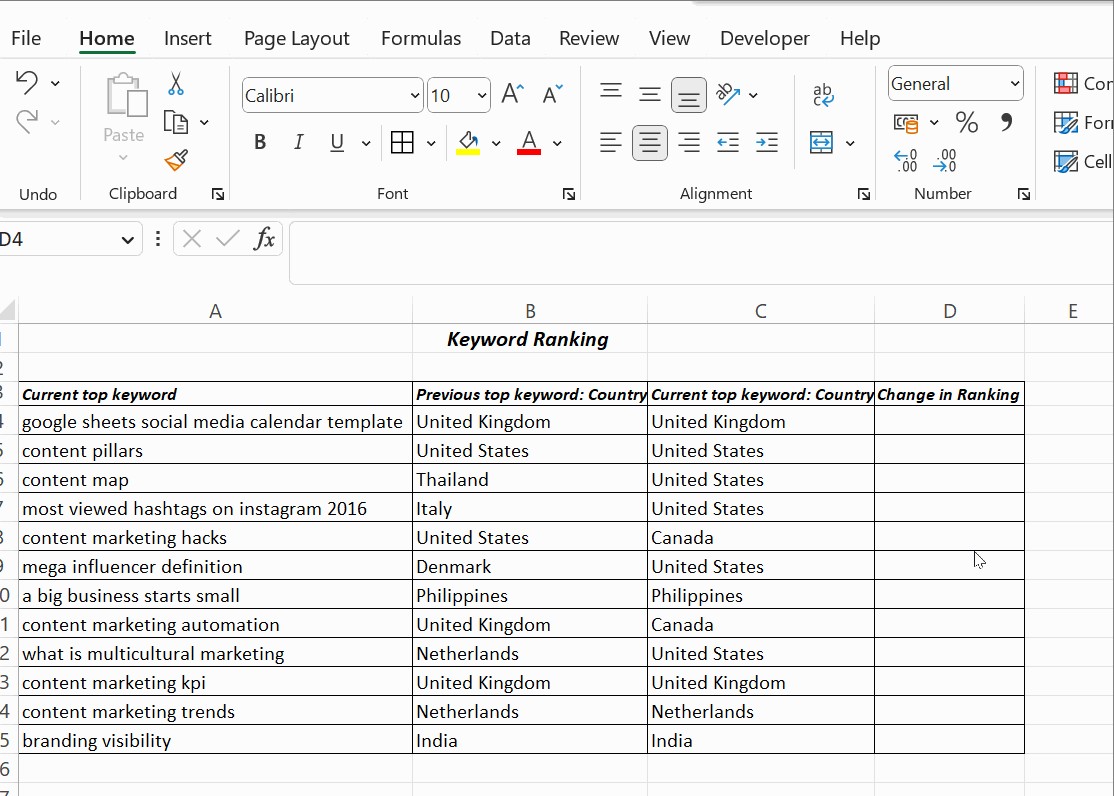
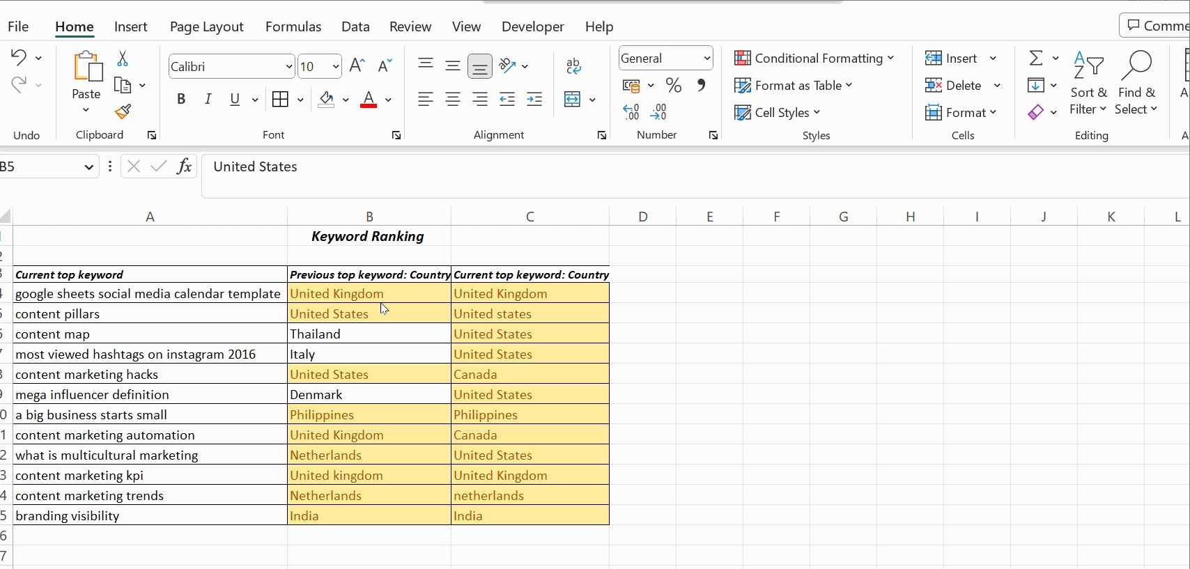
6. Conditional Formatting: Highlighting Differences and Duplicates
Conditional formatting is a powerful feature in Excel that allows you to highlight cells based on specific criteria. This method is particularly useful for visually identifying differences and duplicates in your data.
6.1 How to Use Conditional Formatting
To use conditional formatting, follow these steps:
-
Open your Excel sheet: Launch Microsoft Excel and open the spreadsheet containing the data you want to compare.
-
Select the columns: Select the columns you want to compare. You can select multiple columns by clicking and dragging your mouse.
-
Go to Conditional Formatting: On the Home tab, click Conditional Formatting.
-
Choose a rule: Select a rule based on what you want to highlight.
- Highlight Duplicate Values: To highlight values that appear in both columns, select Highlight Cells Rules > Duplicate Values.
- Highlight Unique Values: To highlight values that appear only in one of the columns, select Highlight Cells Rules > Unique Values.
-
Choose formatting: In the dialog box, choose the formatting you want to apply to the highlighted cells. You can select a predefined format or create a custom format.
-
Apply the formatting: Click OK to apply the conditional formatting.
6.2 Example: Highlighting Duplicate Values
Suppose you want to highlight names that appear in both column A and column B:
- Select columns A and B.
- Go to Home > Conditional Formatting > Highlight Cells Rules > Duplicate Values.
- Choose a formatting style (e.g., light red fill with dark red text).
- Click OK.
Excel will highlight all names that appear in both columns with the selected formatting.
6.3 Example: Highlighting Unique Values
Suppose you want to highlight names that appear only in column A or column B:
- Select columns A and B.
- Go to Home > Conditional Formatting > Highlight Cells Rules > Unique Values.
- Choose a formatting style (e.g., green fill with dark green text).
- Click OK.
Excel will highlight all names that appear only in one of the columns with the selected formatting.
6.4 Using Formulas with Conditional Formatting
You can also use formulas to create more complex conditional formatting rules. For example, you can highlight rows where the values in two columns are different:
- Select the range of cells you want to format.
- Go to Home > Conditional Formatting > New Rule.
- Select Use a formula to determine which cells to format.
- Enter the formula
=A1<>B1(adjust the cell references as needed). - Click Format to choose the formatting style.
- Click OK to apply the rule.
6.5 Advantages
- Visual identification: Conditional formatting provides a visual way to identify patterns and anomalies in your data.
- Easy to use: The user-friendly interface makes it easy to create and apply conditional formatting rules.
- Customizable: You can customize the formatting style to suit your needs.
- Dynamic: Conditional formatting automatically updates as the data changes.
6.6 Limitations
- Limited to visual cues: Conditional formatting only provides visual cues and does not return specific values.
- Can slow down large spreadsheets: Applying conditional formatting to large spreadsheets can slow down performance.
- Not suitable for complex comparisons: Conditional formatting is best suited for simple comparisons.
7. Using LOOKUP Functions to Compare Data
LOOKUP functions in Excel are powerful tools for comparing data across different columns or sheets. These functions allow you to search for a specific value in one column and return a corresponding value from another column.
7.1 VLOOKUP Function
The VLOOKUP function searches for a value in the first column of a range and returns a value from a column to the right.
Syntax: =VLOOKUP(lookup_value, table_array, col_index_num, [range_lookup])
lookup_value: The value you want to search for.table_array: The range of cells where you want to search.col_index_num: The column number in the range from which to return a value.[range_lookup]: Optional. TRUE for approximate match, FALSE for exact match.
Example: To compare values in column A with values in column B and return “Match” or “Not Match”:
- Open your Excel sheet: Launch Microsoft Excel and open the spreadsheet containing the data you want to compare.
- Select an empty column: Choose a column where you want to display the comparison results.
- Enter the formula: In the first cell of the empty column, enter the formula
=IF(ISERROR(VLOOKUP(A1, B:B, 1, FALSE)), "Not Match", "Match"), replacingA1with the first cell you want to compare. - Drag the formula down: Click on the bottom-right corner of the cell containing the formula (the fill handle) and drag it down to apply the formula to all rows in the column.
- Review the results: Excel will display “Match” for rows where the values in column A are found in column B, and “Not Match” where they are not.
7.2 XLOOKUP Function
The XLOOKUP function is a more advanced version of VLOOKUP and HLOOKUP. It can search in both vertical and horizontal ranges and offers more flexibility and features.
Syntax: =XLOOKUP(lookup_value, lookup_array, return_array, [if_not_found], [match_mode], [search_mode])
lookup_value: The value you want to search for.lookup_array: The range of cells where you want to search.return_array: The range of cells from which to return a value.[if_not_found]: Optional. The value to return if no match is found.[match_mode]: Optional. Specifies the type of match.[search_mode]: Optional. Specifies the search direction.
Example: To compare values in column A with values in column B and return “Match” or “Not Match”:
- Open your Excel sheet: Launch Microsoft Excel and open the spreadsheet containing the data you want to compare.
- Select an empty column: Choose a column where you want to display the comparison results.
- Enter the formula: In the first cell of the empty column, enter the formula
=XLOOKUP(A1, B:B, B:B, "Not Match", 0), replacingA1with the first cell you want to compare. - Drag the formula down: Click on the bottom-right corner of the cell containing the formula (the fill handle) and drag it down to apply the formula to all rows in the column.
- Review the results: Excel will display the matching value from column B if found, or “Not Match” if not found.
7.3 Advantages
- Versatile: LOOKUP functions can be used to compare data across different columns or sheets.
- Flexible: XLOOKUP offers more flexibility and features than VLOOKUP.
- Efficient: LOOKUP functions are efficient for finding matching values in large datasets.
7.4 Limitations
- Requires understanding of syntax: LOOKUP functions can be complex and require an understanding of their syntax.
- Can be slow on very large datasets: LOOKUP functions can be slow on very large datasets.
- Exact match may be required: Depending on the settings, LOOKUP functions may require an exact match.
8. Step-by-Step Guide: Comparing Data in Excel
Here’s a consolidated step-by-step guide that encompasses various methods to compare data in Excel effectively.
8.1 Preparation
- Open your Excel sheet: Launch Microsoft Excel and open the spreadsheet containing the data you want to compare.
- Identify columns for comparison: Determine which columns you need to compare and what type of comparison you want to perform (e.g., exact match, case-sensitive, identifying duplicates).
- Choose an output column: Select an empty column where you want to display the comparison results.
8.2 Using the Equals Operator (=)
- Enter the formula: In the first cell of the output column, enter the formula
=A1=B1, replacingA1andB1with the first cells you want to compare. - Drag the formula down: Click on the bottom-right corner of the cell containing the formula (the fill handle) and drag it down to apply the formula to all rows in the column.
- Review the results: Excel will display
TRUEif the values match andFALSEif they don’t.
8.3 Using the IF Condition
- Enter the formula: In the first cell of the output column, enter the formula
=IF(A1=B1, "Match", "Not Match"), replacingA1andB1with the first cells you want to compare. - Drag the formula down: Apply the formula to all rows in the column by dragging the fill handle.
- Review the results: Excel will display “Match” for rows where the values match and “Not Match” where they don’t.
8.4 Using the EXACT() Function
- Enter the formula: In the first cell of the output column, enter the formula
=IF(EXACT(A1, B1), "Match", "Not Match")for a case-sensitive comparison. - Drag the formula down: Apply the formula to all rows.
- Review the results: Excel will display “Match” only if the values match exactly, including case.
8.5 Using Conditional Formatting
- Select the columns: Select the columns you want to compare.
- Go to Conditional Formatting: On the Home tab, click Conditional Formatting.
- Highlight Duplicate Values: Select Highlight Cells Rules > Duplicate Values to highlight values that appear in both columns.
- Highlight Unique Values: Select Highlight Cells Rules > Unique Values to highlight values that appear only in one of the columns.
- Choose formatting: Choose the formatting you want to apply to the highlighted cells and click OK.
8.6 Using LOOKUP Functions (VLOOKUP/XLOOKUP)
- Enter the formula: In the first cell of the output column, enter the appropriate LOOKUP formula (e.g.,
=IF(ISERROR(VLOOKUP(A1, B:B, 1, FALSE)), "Not Match", "Match")for VLOOKUP or=XLOOKUP(A1, B:B, B:B, "Not Match", 0)for XLOOKUP). - Drag the formula down: Apply the formula to all rows.
- Review the results: Excel will display the matching result or “Not Match” if no match is found.
8.7 Final Steps
- Review the results: Carefully review the results of your comparison.
- Filter and sort: Use Excel’s filtering and sorting capabilities to further analyze the data.
- Address discrepancies: Investigate and address any discrepancies or errors identified during the comparison.
By following this comprehensive guide, you can efficiently and accurately compare data in Excel using a variety of methods tailored to your specific needs.
9. FAQ: Common Questions About Comparing Data in Excel
Here are some frequently asked questions about comparing data in Excel:
9.1 How do I compare two columns for differences?
You can use the IF condition with the <> operator to check for differences. The formula would be =IF(A1<>B1, "Different", "Same").
9.2 How can I perform a case-sensitive comparison?
Use the EXACT() function to perform a case-sensitive comparison. The formula would be =IF(EXACT(A1, B1), "Match", "Not Match").
9.3 How do I highlight duplicate values in two columns?
Use conditional formatting to highlight duplicate values. Select the columns, go to Home > Conditional Formatting > Highlight Cells Rules > Duplicate Values, and choose the desired formatting.
9.4 How do I compare data across multiple sheets?
You can use LOOKUP functions like VLOOKUP or XLOOKUP to compare data across multiple sheets. Reference the range in the other sheet in the formula.
9.5 How do I ignore errors when comparing data?
Use the IFERROR function to handle errors. For example, =IFERROR(IF(A1=B1, "Match", "Not Match"), "Error") will return “Error” if there is an error in the comparison.
9.6 How can I compare two lists and find missing items?
Use the XLOOKUP function with the if_not_found argument to find missing items. For example, =XLOOKUP(A1, B:B, B:B, "Missing", 0) will return “Missing” if the value in A1 is not found in column B.
9.7 How to compare two columns in Excel and return value from third column?
To compare two columns and return a value from a third column, you can use a combination of the IF function and the INDEX function. Here’s how:
Scenario: You have three columns: Column A contains IDs, Column B contains corresponding names, and Column C contains statuses. You want to compare IDs in Column A with another list of IDs in Column D and, if there’s a match, return the status from Column C.
Steps:
-
Set up your data:
- Column A: IDs
- Column B: Names (corresponding to IDs in Column A)
- Column C: Statuses (corresponding to IDs in Column A)
- Column D: List of IDs to compare against Column A
- Column E: Where you want to return the status if there’s a match
-
Enter the formula in Column E:
In cell
E1, enter the following formula:=IF(ISNUMBER(MATCH(D1,A:A,0)), INDEX(C:C, MATCH(D1,A:A,0)), "No Match")MATCH(D1,A:A,0): This part of the formula looks for the value in cellD1within the entire Column A. The0signifies that it’s looking for an exact match. If it finds a match, it returns the row number where the match was found. If it doesn’t find a match, it returns an error (#N/A).ISNUMBER(MATCH(D1,A:A,0)): This checks if the result of theMATCHfunction is a number (i.e., a row number where a match was found). IfMATCHfinds a match,ISNUMBERreturnsTRUE; otherwise, it returnsFALSE.INDEX(C:C, MATCH(D1,A:A,0)): IfMATCHfinds a match (and thusISNUMBERreturnsTRUE), this part of the formula uses theINDEXfunction to return the corresponding value from Column C. TheMATCHfunction provides the row number toINDEX, so it knows which cell in Column C to return.IF(ISNUMBER(MATCH(D1,A:A,0)), ... , "No Match"): This is the mainIFfunction. IfISNUMBERreturnsTRUE(i.e., a match is found), it performs theINDEXfunction to return the status from Column C. IfISNUMBERreturnsFALSE(i.e., no match is found), it returns"No Match".
-
Drag the formula down:
Click on the bottom-right corner of cell
E1(the fill handle) and drag it down to apply the formula to all rows in Column E, corresponding to the list of IDs in Column D. -
Review the results:
Column E will now display the status from Column C for each ID in Column D that matches an ID in Column A. If there is no match, it will display
"No Match".
9.8 How to compare two columns in Google Sheets?
Here are several methods to compare two columns in Google Sheets:
-
Using the
IFFunction:This is similar to Excel. You can use the
IFfunction to compare two columns row by row and return a specified result if the values match or don’t match.-
Formula:
=IF(A1=B1, "Match", "No Match")In this formula,
A1andB1are the first cells in the columns you want to compare. Drag this formula down to apply it to the rest of the rows. -
Steps:
- Open your Google Sheet and select an empty column where you want to display the results.
- In the first cell of the empty column, enter the formula
=IF(A1=B1, "Match", "No Match"). - Drag the fill handle (the small square at the bottom-right of the cell) down to apply the formula to all rows.
- Review the results; the column will display “Match” if the values in the corresponding rows of the compared columns are the same, and “No Match” if they are different.
-
-
Using Conditional Formatting:
Conditional formatting can highlight cells based on whether they match or don’t match.
-
Steps:
- Select the range of cells you want to compare (e.g.,
A1:B100). - Go to “Format” > “Conditional formatting.”
- Under “Format rules,” choose “Custom formula is” in the “Format cells if” dropdown.
- Enter the formula
=A1=B1(assumingA1is the first cell in your selected range). - Choose the formatting style (e.g., background color) to apply when the condition is true (i.e., the cells match).
- Click “Done.”
- Add another rule if you want to format cells that don’t match. Use the formula
=A1<>B1and choose a different formatting style.
- Select the range of cells you want to compare (e.g.,
-
-
Using the
EXACTFunction for Case-Sensitive Comparison:The
EXACTfunction compares two strings and returnsTRUEif they are exactly the same, including case.-
Formula:
=EXACT(A1, B1) -
Steps:
- Select an empty column where you want to display the results.
- In the first cell of the empty column, enter the formula
=EXACT(A1, B1). - Drag the fill handle down to apply the formula to all rows.
- Review the results; the column will display
TRUEif the values in the corresponding rows are exactly the same (including case), andFALSEif they are different.
-
-
Using
QUERYfor More Complex Comparisons:The
QUERYfunction can be used for more complex comparisons, such as finding values that exist in one column but not in another.-
Example: To find values in Column A that are not in Column B, you can use a helper column.
-
In a helper column (e.g., Column C), enter the formula:
=IF(ISERROR(MATCH(A1, B:B, 0)), A1, "")This formula checks if the value in
A1exists in Column B. If it does not, it returns the value fromA1; otherwise, it returns an empty string. -
Drag the fill handle down to apply the formula to all rows.
-
Filter Column C to show only non-empty values; these are the values that exist in Column A but not in Column B.
-
-
-
Using Array Formulas:
Array formulas can perform operations on entire arrays (columns) at once.
- **Example