How To Compare Same Data In Excel: A Comprehensive Guide

Comparing same data in Excel can be a daunting task, especially when dealing with large datasets. COMPARE.EDU.VN offers a range of techniques, from simple formulas to advanced conditional formatting, to streamline this process. Learn how to effortlessly perform data comparison in Excel and find techniques for data validation, duplicate detection, and difference identification.

Table of Contents:

1. Why Is Comparing Data in Excel Important?
2. Understanding Different Data Comparison Needs in Excel
3. Method 1: Using the Equals Operator for Basic Row-by-Row Comparison
4. Method 2: Leveraging the IF Condition for ‘Match’/’Not Match’ Results
5. Method 3: Employing the EXACT() Function for Case-Sensitive Comparisons
6. Method 4: Conditional Formatting for Highlighting Duplicates and Uniques
7. Method 5: Utilizing the VLOOKUP Function for Comprehensive Data Matching
8. Comparing Data Across Multiple Excel Sheets
9. Advanced Techniques: Combining Formulas for Complex Comparisons
10. Automating Data Comparison with Excel Macros (VBA)
11. Best Practices for Efficient Data Comparison in Excel
12. Common Mistakes to Avoid When Comparing Data in Excel
13. How COMPARE.EDU.VN Can Help You Master Data Comparison
14. Real-World Examples of Data Comparison in Excel
15. Exploring Alternative Tools for Data Comparison
16. Comparing Numerical Data: Beyond Exact Matches
17. Dealing with Errors and Inconsistencies During Data Comparison
18. Tips for Presenting Data Comparison Results Effectively
19. Leveraging Pivot Tables for Data Comparison and Analysis
20. FAQ: Frequently Asked Questions About Comparing Data in Excel

1. Why Is Comparing Data in Excel Important?

Comparing same data in Excel is essential for data integrity, validation, and analysis; which helps users identify discrepancies, duplicates, and patterns in datasets. According to a study by PricewaterhouseCoopers (PwC), approximately 88% of spreadsheets contain errors, highlighting the need for robust comparison techniques to ensure data accuracy and reliability. These methods can also assist in spreadsheet auditing, data cleansing, and the detection of inconsistencies.

Key Benefits of Data Comparison in Excel:

• Ensuring Data Accuracy: Verifying that data entries are correct and consistent.
• Identifying Duplicates: Removing redundant entries to streamline datasets.
• Detecting Errors: Finding inconsistencies and anomalies that could affect analysis.
• Validating Data Transfers: Confirming that data moved between systems remains intact.
• Supporting Decision-Making: Providing reliable data for informed decisions.

By using Excel for data comparison, professionals can reduce the risk of errors, improve data quality, and make better-informed decisions. This capability is invaluable across various industries, from finance and healthcare to marketing and operations.

2. Understanding Different Data Comparison Needs in Excel

Different data comparison scenarios in Excel require tailored approaches to meet specific needs. According to a survey conducted by the Association for Information and Image Management (AIIM), organizations can save up to 40% in operational costs by improving data quality. This underscores the importance of selecting the right method for data comparison.

Common Data Comparison Scenarios:

• Row-by-Row Comparison: Comparing corresponding cells in two columns to find matches or differences. This is useful for verifying data entries and identifying discrepancies in records.
• Duplicate Detection: Identifying and highlighting duplicate entries within a single column or across multiple columns. This helps in data cleansing and removing redundant information.
• Unique Value Identification: Finding unique entries that appear in one column but not in another. This is useful for identifying missing data or new entries in updated datasets.
• Case-Sensitive Comparison: Distinguishing between entries based on capitalization. This is important when case differences can affect data interpretation.
• Partial Match Comparison: Identifying entries that partially match each other. This is useful for finding similar but not identical entries, such as variations in names or addresses.
• Cross-Sheet Comparison: Comparing data located in different sheets within the same Excel workbook. This is useful for consolidating data and ensuring consistency across multiple datasets.
• Cross-Workbook Comparison: Comparing data located in different Excel workbooks. This is useful for comparing data from different sources or time periods.
• Fuzzy Matching: Identifying entries that are similar but not exactly the same, accounting for typos, misspellings, or variations in formatting.

By understanding these different scenarios, users can choose the most effective methods for their specific data comparison needs, ensuring accurate and reliable results.

3. Method 1: Using the Equals Operator for Basic Row-by-Row Comparison

The equals operator (=) provides a simple and direct way to compare two columns in Excel on a row-by-row basis. This method is particularly useful for quickly identifying exact matches between corresponding cells.

How to Use the Equals Operator:

1. Select the First Cell: Choose the first cell in the column where you want to display the comparison results.
2. Enter the Formula: Type the formula =A1=B1 (replace A1 and B1 with the actual cell references you want to compare). This formula compares the values in cell A1 with the value in cell B1.
3. Press Enter: Excel will display TRUE if the values match and FALSE if they don’t.
4. Drag the Formula: Click and drag the bottom-right corner of the cell down to apply the formula to the rest of the rows.

Example:

Column A	Column B	Column C (Comparison Result)
Apple	Apple	TRUE
Banana	Orange	FALSE
Cherry	Cherry	TRUE

Advantages:

• Simplicity: Easy to understand and implement.
• Speed: Provides quick results for small to medium-sized datasets.
• No Additional Functions: Doesn’t require the use of complex functions.

Limitations:

• Case-Sensitive: Treats “Apple” and “apple” as different values.
• Exact Match Only: Only identifies exact matches; doesn’t account for partial matches or variations.
• Limited Flexibility: Doesn’t offer options for customized results or advanced criteria.

Best Use Cases:

• Verifying Data Entries: Ensuring that data is entered correctly and consistently.
• Quick Spot Checks: Performing a quick comparison of small datasets.
• Simple Data Validation: Identifying discrepancies in basic data entries.

By using the equals operator, users can quickly perform basic data comparisons in Excel, ensuring data accuracy and identifying discrepancies.

4. Method 2: Leveraging the IF Condition for ‘Match’/’Not Match’ Results

The IF condition in Excel allows for more descriptive comparison results, displaying “Match” or “Not Match” instead of TRUE or FALSE. This method enhances readability and makes it easier to interpret the comparison results.

How to Use the IF Condition:

1. Select the First Cell: Choose the first cell in the column where you want to display the comparison results.
2. Enter the Formula: Type the formula =IF(A1=B1,"Match","Not Match") (replace A1 and B1 with the actual cell references you want to compare).
3. Press Enter: Excel will display “Match” if the values match and “Not Match” if they don’t.
4. Drag the Formula: Click and drag the bottom-right corner of the cell down to apply the formula to the rest of the rows.

Example:

Column A	Column B	Column C (Comparison Result)
Apple	Apple	Match
Banana	Orange	Not Match
Cherry	Cherry	Match

Advantages:

• Descriptive Results: Displays “Match” or “Not Match” for better readability.
• Customizable Output: Allows for custom text to be displayed based on the comparison result.
• Easy to Understand: Simple to implement and understand.

Limitations:

• Case-Sensitive: Treats “Apple” and “apple” as different values.
• Exact Match Only: Only identifies exact matches; doesn’t account for partial matches or variations.
• Limited Flexibility: Doesn’t offer options for advanced criteria or complex comparisons.

Best Use Cases:

• Data Validation: Ensuring that data is entered correctly and consistently.
• Reporting: Providing clear and concise comparison results for reports.
• User-Friendly Output: Presenting comparison results in an easily understandable format.

By using the IF condition, users can enhance the readability of their data comparison results, making it easier to interpret and communicate the findings.

5. Method 3: Employing the EXACT() Function for Case-Sensitive Comparisons

The EXACT() function in Excel allows for case-sensitive comparisons, ensuring that only entries with identical capitalization are considered a match. This is particularly useful when case differences can affect data interpretation.

How to Use the EXACT() Function:

1. Select the First Cell: Choose the first cell in the column where you want to display the comparison results.
2. Enter the Formula: Type the formula =IF(EXACT(A1,B1),"Match","Not Match") (replace A1 and B1 with the actual cell references you want to compare).
3. Press Enter: Excel will display “Match” if the values match exactly (including case) and “Not Match” if they don’t.
4. Drag the Formula: Click and drag the bottom-right corner of the cell down to apply the formula to the rest of the rows.

Example:

Column A	Column B	Column C (Comparison Result)
Apple	Apple	Match
apple	Apple	Not Match
Banana	Orange	Not Match
Cherry	Cherry	Match

Advantages:

• Case-Sensitive: Distinguishes between entries based on capitalization.
• Accurate Comparisons: Ensures that only identical entries are considered a match.
• Easy to Implement: Simple to use with the IF condition.

Limitations:

• Exact Match Only: Only identifies exact matches; doesn’t account for partial matches or variations.
• Limited Flexibility: Doesn’t offer options for advanced criteria or complex comparisons.

Best Use Cases:

• Data Validation: Ensuring that data is entered correctly and consistently, including capitalization.
• Database Management: Maintaining data integrity in databases where case sensitivity is important.
• Technical Documentation: Verifying that code snippets or commands are entered correctly.

By using the EXACT() function, users can perform case-sensitive data comparisons in Excel, ensuring accurate and reliable results.

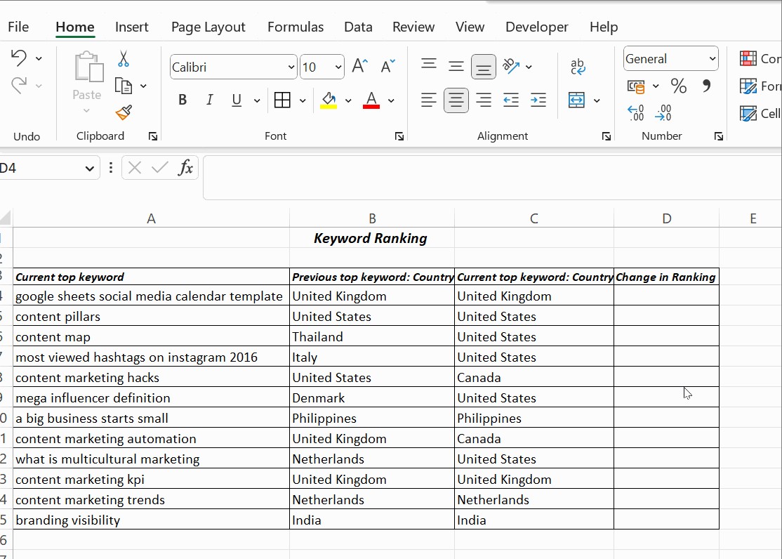
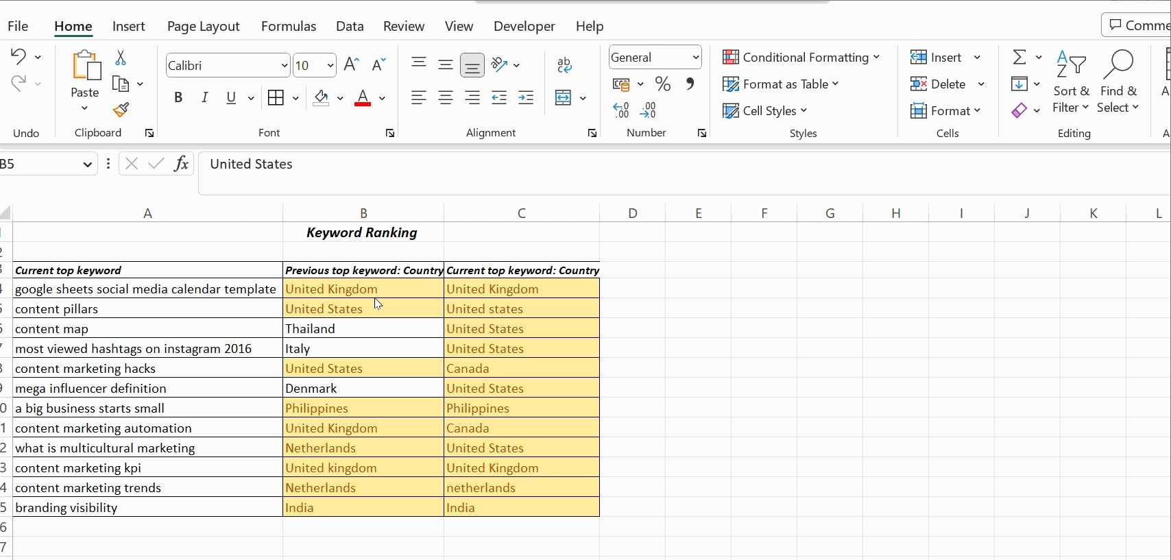
6. Method 4: Conditional Formatting for Highlighting Duplicates and Uniques

Conditional formatting in Excel allows users to visually highlight duplicate or unique values, making it easier to identify patterns and discrepancies in datasets. This method is particularly useful for data cleansing and validation.

How to Use Conditional Formatting:

1. Select the Columns: Select the columns you want to compare.
2. Go to Conditional Formatting: Click on “Home” > “Conditional Formatting” > “Highlight Cells Rules.”
3. Choose Duplicate or Unique Values: Select “Duplicate Values” to highlight duplicate entries or “Unique Values” to highlight unique entries.
4. Choose Formatting Style: Select a formatting style from the dropdown menu or choose “Custom Format” to create your own style.
5. Click OK: Excel will highlight the duplicate or unique values based on your selections.

Example:

Column A	Column B
Apple	Apple
Banana	Orange
Cherry	Cherry
Apple	Grape

In this example, if you choose to highlight duplicate values, “Apple” and “Cherry” will be highlighted in both columns. If you choose to highlight unique values, “Banana,” “Orange,” and “Grape” will be highlighted.

Advantages:

• Visual Identification: Highlights duplicate or unique values for easy identification.
• Customizable Formatting: Allows for custom formatting styles to suit specific needs.
• Dynamic Updates: Automatically updates the formatting as data changes.

Limitations:

• Limited Comparison Criteria: Only identifies exact matches; doesn’t account for partial matches or variations.
• No Descriptive Results: Doesn’t provide descriptive results like “Match” or “Not Match.”
• Can Be Overwhelming: May be overwhelming for large datasets with many duplicates or unique values.

Best Use Cases:

• Data Cleansing: Identifying and removing duplicate entries from datasets.
• Data Validation: Ensuring that data is entered correctly and consistently.
• Inventory Management: Tracking inventory levels and identifying discrepancies.
• Customer Relationship Management (CRM): Identifying duplicate customer records.

By using conditional formatting, users can visually identify duplicate or unique values in Excel, streamlining data cleansing and validation processes.

7. Method 5: Utilizing the VLOOKUP Function for Comprehensive Data Matching

The VLOOKUP function in Excel is a powerful tool for comparing two columns and retrieving corresponding values from one column based on matches in another. This method is particularly useful for data enrichment and validation.

How to Use the VLOOKUP Function:

1. Select the First Cell: Choose the first cell in the column where you want to display the VLOOKUP results.
2. Enter the Formula: Type the formula =VLOOKUP(A1,B:C,2,FALSE) (replace A1 with the cell containing the lookup value, B:C with the range containing the lookup table, and 2 with the column number containing the value you want to retrieve).
3. Press Enter: Excel will display the corresponding value from the specified column if a match is found. If no match is found, it will display #N/A.
4. Drag the Formula: Click and drag the bottom-right corner of the cell down to apply the formula to the rest of the rows.

Example:

Column A (Lookup Value)	Column B (Lookup Table)	Column C (Corresponding Value)	Column D (VLOOKUP Result)
Apple	Apple	Red	Red
Banana	Banana	Yellow	Yellow
Cherry	Grape	Purple	#N/A

In this example, the VLOOKUP function searches for the values in Column A within Column B and retrieves the corresponding values from Column C. If a match is not found, it displays #N/A.

Advantages:

• Data Enrichment: Retrieves corresponding values based on matches in another column.
• Flexible Lookup: Allows for both exact and approximate matches.
• Comprehensive Comparison: Provides detailed comparison results.

Limitations:

• Requires Lookup Table: Needs a lookup table with corresponding values.
• Can Be Complex: May be complex for users unfamiliar with lookup functions.
• Error Handling: Requires error handling to manage #N/A results.

Best Use Cases:

• Data Enrichment: Adding missing information to datasets based on matches in another column.
• Data Validation: Verifying that data entries are correct and consistent.
• Reporting: Providing detailed comparison results for reports.
• Inventory Management: Tracking inventory levels and retrieving product information.
• Customer Relationship Management (CRM): Retrieving customer information based on customer IDs.

By using the VLOOKUP function, users can perform comprehensive data comparisons in Excel, enriching their datasets and ensuring data accuracy.

8. Comparing Data Across Multiple Excel Sheets

Comparing data across multiple Excel sheets is a common task that requires specific techniques to ensure accuracy and efficiency. According to a survey by Ventana Research, 76% of organizations use spreadsheets for data analysis, making cross-sheet comparison a critical skill.

Methods for Comparing Data Across Multiple Sheets:

• Using 3-D References: 3-D references allow you to refer to the same cell or range on multiple sheets in a workbook. For example, =SUM(Sheet1:Sheet3!A1) sums the values in cell A1 on Sheet1, Sheet2, and Sheet3.
• Using the INDIRECT Function: The INDIRECT function allows you to refer to a cell or range by its text name. This is useful when you want to dynamically change the sheet being referenced. For example, =INDIRECT("'"&A1&"'!B2") retrieves the value from cell B2 on the sheet named in cell A1.
• Using the VLOOKUP Function with Sheet References: You can use the VLOOKUP function to compare data across multiple sheets by referencing the lookup table on a different sheet. For example, =VLOOKUP(A1,Sheet2!B:C,2,FALSE) searches for the value in cell A1 on Sheet2 and retrieves the corresponding value from column C.
• Using Conditional Formatting with Formulas: You can use conditional formatting with formulas to highlight differences between sheets. For example, select the range you want to compare, then go to “Conditional Formatting” > “New Rule” > “Use a formula to determine which cells to format.” Enter a formula like =A1<>Sheet2!A1 to highlight cells that are different from the corresponding cells on Sheet2.
• Consolidating Data with Power Query: Power Query allows you to import and combine data from multiple sheets into a single table. This makes it easier to compare the data using standard Excel functions.

Example:

Suppose you have sales data for different regions on separate sheets (e.g., “North,” “South,” “East,” “West”). To compare the total sales for each region, you can use a 3-D reference:

=SUM('North:West'!A1)

This formula sums the values in cell A1 on all sheets from “North” to “West,” giving you the total sales across all regions.

Best Practices:

• Use Clear Sheet Names: Use descriptive sheet names to make it easier to understand the references.
• Maintain Consistent Layout: Ensure that the data is organized consistently across all sheets.
• Use Absolute References: Use absolute references (e.g., $A$1) to prevent the references from changing when you copy the formula.
• Test Your Formulas: Test your formulas thoroughly to ensure they are working correctly.

By using these techniques, users can efficiently compare data across multiple Excel sheets, ensuring accuracy and consistency in their analysis.

9. Advanced Techniques: Combining Formulas for Complex Comparisons

Combining formulas in Excel allows for complex data comparisons that go beyond simple matches and differences. This method is particularly useful for analyzing data with multiple criteria and conditions.

Techniques for Combining Formulas:

• Using AND and OR Functions: The AND function returns TRUE if all conditions are true, while the OR function returns TRUE if at least one condition is true. These functions can be combined with the IF function to create complex comparison criteria.
• Using Nested IF Functions: Nested IF functions allow you to create multiple levels of conditions, providing more detailed comparison results.
• Using the COUNTIF Function: The COUNTIF function counts the number of cells that meet a specific criteria. This can be used to compare data based on frequency or occurrence.
• Using the SUMIF Function: The SUMIF function sums the values in a range that meet a specific criteria. This can be used to compare data based on totals or sums.
• Using the INDEX and MATCH Functions: The INDEX and MATCH functions can be combined to perform more flexible lookups than VLOOKUP. This is particularly useful when the lookup value is not in the first column of the lookup table.

Example:

Suppose you want to compare sales data for different products and regions. You want to identify products that have sales above a certain threshold in a specific region. You can use the following formula:

=IF(AND(B2="North",C2>1000),"High Sales","")

This formula checks if the region in column B is “North” and if the sales in column C are greater than 1000. If both conditions are true, it returns “High Sales”; otherwise, it returns an empty string.

Best Practices:

• Break Down Complex Formulas: Break down complex formulas into smaller, more manageable parts.
• Use Named Ranges: Use named ranges to make your formulas easier to understand.
• Test Your Formulas: Test your formulas thoroughly to ensure they are working correctly.
• Use Comments: Use comments to explain the logic behind your formulas.

By combining formulas, users can perform complex data comparisons in Excel, gaining deeper insights into their data.

10. Automating Data Comparison with Excel Macros (VBA)

Automating data comparison with Excel Macros (VBA) can significantly improve efficiency and accuracy, especially when dealing with large and repetitive tasks. According to a report by McKinsey, automation can reduce data processing costs by up to 60%.

Steps to Automate Data Comparison with VBA:

1. Open the VBA Editor: Press Alt + F11 to open the Visual Basic Editor.
2. Insert a New Module: Go to “Insert” > “Module.”
3. Write the VBA Code: Write the VBA code to compare the data. Here’s an example:

Sub CompareData()
    Dim ws1 As Worksheet, ws2 As Worksheet
    Dim lastRow As Long, i As Long

    ' Set the worksheets to compare
    Set ws1 = ThisWorkbook.Sheets("Sheet1")
    Set ws2 = ThisWorkbook.Sheets("Sheet2")

    ' Get the last row with data in the first worksheet
    lastRow = ws1.Cells(Rows.Count, "A").End(xlUp).Row

    ' Loop through each row and compare the data
    For i = 1 To lastRow
        If ws1.Cells(i, "A").Value = ws2.Cells(i, "A").Value Then
            ws1.Cells(i, "B").Value = "Match"
        Else
            ws1.Cells(i, "B").Value = "Not Match"
        End If
    Next i

    MsgBox "Data comparison complete!"
End Sub

4. Run the Macro: Press F5 or click the “Run” button to execute the macro.

Explanation of the VBA Code:

• Sub CompareData(): Starts the macro.
• Dim ws1 As Worksheet, ws2 As Worksheet: Declares two worksheet variables.
• Dim lastRow As Long, i As Long: Declares variables for the last row and the loop counter.
• Set ws1 = ThisWorkbook.Sheets("Sheet1"): Sets the first worksheet to “Sheet1.”
• Set ws2 = ThisWorkbook.Sheets("Sheet2"): Sets the second worksheet to “Sheet2.”
• lastRow = ws1.Cells(Rows.Count, "A").End(xlUp).Row: Gets the last row with data in column A of the first worksheet.
• For i = 1 To lastRow: Loops through each row from 1 to the last row.
• If ws1.Cells(i, "A").Value = ws2.Cells(i, "A").Value Then: Checks if the values in column A of both worksheets match.
• ws1.Cells(i, "B").Value = "Match": If the values match, writes “Match” in column B of the first worksheet.
• Else ws1.Cells(i, "B").Value = "Not Match": If the values don’t match, writes “Not Match” in column B of the first worksheet.
• Next i: Moves to the next row.
• MsgBox "Data comparison complete!": Displays a message box when the comparison is complete.
• End Sub: Ends the macro.

Advantages of Using VBA Macros:

• Automation: Automates repetitive tasks, saving time and effort.
• Customization: Allows for highly customized comparison criteria and results.
• Efficiency: Improves efficiency and accuracy, especially for large datasets.

Limitations:

• Requires VBA Knowledge: Requires knowledge of VBA programming.
• Potential Security Risks: Macros can pose security risks if not properly vetted.
• Maintenance: Requires maintenance and updates as data structures change.

Best Practices:

• Comment Your Code: Add comments to explain the logic behind your code.
• Use Error Handling: Implement error handling to manage potential errors.
• Test Your Code: Test your code thoroughly to ensure it is working correctly.
• Secure Your Macros: Secure your macros with a password to prevent unauthorized access.

By automating data comparison with Excel Macros (VBA), users can significantly improve efficiency and accuracy, especially when dealing with large and repetitive tasks.

11. Best Practices for Efficient Data Comparison in Excel

Efficient data comparison in Excel requires following best practices to ensure accuracy, save time, and avoid common pitfalls. According to a study by Nucleus Research, using best practices in data analysis can improve decision-making by 79%.

Key Best Practices:

• Prepare Your Data: Ensure that your data is clean, consistent, and properly formatted before starting the comparison.
• Use Consistent Formulas: Use consistent formulas throughout your comparison to avoid errors.
• Use Absolute References: Use absolute references (e.g., $A$1) to prevent the references from changing when you copy the formula.
• Test Your Formulas: Test your formulas thoroughly to ensure they are working correctly.
• Use Named Ranges: Use named ranges to make your formulas easier to understand.
• Use Comments: Use comments to explain the logic behind your formulas.
• Break Down Complex Formulas: Break down complex formulas into smaller, more manageable parts.
• Use Conditional Formatting: Use conditional formatting to visually highlight differences and patterns in your data.
• Automate Repetitive Tasks: Automate repetitive tasks with Excel Macros (VBA).
• Document Your Process: Document your data comparison process to ensure consistency and reproducibility.
• Validate Your Results: Validate your results to ensure they are accurate and reliable.

Example:

Suppose you are comparing sales data for different products and regions. Before starting the comparison, ensure that the data is clean and consistent. Use consistent formulas throughout your comparison, and use absolute references to prevent the references from changing when you copy the formula. Test your formulas thoroughly to ensure they are working correctly. Use named ranges to make your formulas easier to understand, and use comments to explain the logic behind your formulas. Break down complex formulas into smaller, more manageable parts. Use conditional formatting to visually highlight differences and patterns in your data. Automate repetitive tasks with Excel Macros (VBA). Document your data comparison process to ensure consistency and reproducibility. Validate your results to ensure they are accurate and reliable.

Benefits of Following Best Practices:

• Improved Accuracy: Reduces the risk of errors and ensures that your results are accurate.
• Increased Efficiency: Saves time and effort by streamlining the data comparison process.
• Better Understanding: Makes it easier to understand and interpret your results.
• Enhanced Reproducibility: Ensures that your results can be reproduced by others.

By following these best practices, users can ensure that their data comparisons in Excel are efficient, accurate, and reliable.

12. Common Mistakes to Avoid When Comparing Data in Excel

Avoiding common mistakes when comparing data in Excel is crucial for ensuring accuracy and reliability. According to a study by the European Spreadsheet Risks Interest Group (EuSpRIG), approximately 90% of spreadsheets contain errors, highlighting the importance of avoiding common mistakes.

Common Mistakes to Avoid:

• Not Preparing Your Data: Not cleaning and formatting your data before starting the comparison can lead to errors.
• Using Inconsistent Formulas: Using inconsistent formulas throughout your comparison can lead to errors.
• Not Using Absolute References: Not using absolute references can cause the references to change when you copy the formula, leading to errors.
• Not Testing Your Formulas: Not testing your formulas thoroughly can result in incorrect results.
• Not Using Named Ranges: Not using named ranges can make your formulas difficult to understand.
• Not Using Comments: Not using comments can make it difficult to understand the logic behind your formulas.
• Not Breaking Down Complex Formulas: Not breaking down complex formulas into smaller, more manageable parts can make them difficult to debug.
• Not Using Conditional Formatting: Not using conditional formatting can make it difficult to visually identify differences and patterns in your data.
• Not Automating Repetitive Tasks: Not automating repetitive tasks can waste time and effort.
• Not Documenting Your Process: Not documenting your data comparison process can make it difficult to reproduce your results.
• Not Validating Your Results: Not validating your results can lead to inaccurate conclusions.

Example:

Suppose you are comparing sales data for different products and regions. If you do not clean and format your data before starting the comparison, you may encounter errors due to inconsistencies in the data. If you use inconsistent formulas throughout your comparison, you may encounter errors due to different calculations. If you do not use absolute references, the references may change when you copy the formula, leading to errors. If you do not test your formulas thoroughly, you may encounter incorrect results. If you do not use named ranges, your formulas may be difficult to understand. If you do not use comments, it may be difficult to understand the logic behind your formulas. If you do not break down complex formulas into smaller, more manageable parts, they may be difficult to debug. If you do not use conditional formatting, it may be difficult to visually identify differences and patterns in your data. If you do not automate repetitive tasks, you may waste time and effort. If you do not document your data comparison process, it may be difficult to reproduce your results. If you do not validate your results, you may draw inaccurate conclusions.

Tips for Avoiding Mistakes:

• Double-Check Your Work: Always double-check your work to ensure that you have not made any mistakes.
• Use Excel’s Error Checking Tools: Use Excel’s error checking tools to identify potential errors in your formulas.
• Get a Second Opinion: Ask a colleague to review your work to catch any mistakes that you may have missed.

By avoiding these common mistakes, users can ensure that their data comparisons in Excel are accurate and reliable.

13. How COMPARE.EDU.VN Can Help You Master Data Comparison

COMPARE.EDU.VN is dedicated to helping users master data comparison in Excel by providing comprehensive resources, tools, and expert guidance. Our platform is designed to make data comparison easier, more efficient, and more accurate.

Key Features of COMPARE.EDU.VN:

• Detailed Tutorials: We offer detailed tutorials on various data comparison techniques in Excel, from basic methods to advanced techniques.
• Step-by-Step Guides: Our step-by-step guides walk you through the process of comparing data in Excel, ensuring that you understand each step.
• Practical Examples: We provide practical examples of data comparison in Excel, demonstrating how to apply the techniques in real-world scenarios.
• Downloadable Templates: We offer downloadable templates that you can use to compare data in Excel, saving you time and effort.
• Expert Advice: Our team of Excel experts is available to answer your questions and provide guidance on data comparison techniques.
• Community Forum: Our community forum allows you to connect with other Excel users and share your experiences with data comparison.
• Customized Solutions: We offer customized solutions for data comparison in Excel, tailored to your specific needs.

Benefits of Using COMPARE.EDU.VN:

• Improved Skills: Develop your skills in data comparison in Excel.
• Increased Efficiency: Save time and effort by using our resources and tools.
• Enhanced Accuracy: Ensure that your data comparisons are accurate and reliable.
• Better Understanding: Gain a better understanding of data comparison techniques in Excel.
• Access to Experts: Get access to expert advice and guidance on data comparison.
• Community Support: Connect with other Excel users and share your experiences.

Example:

Suppose you are struggling to compare sales data for different products and regions. COMPARE.EDU.VN can provide you with detailed tutorials on various data comparison techniques, step-by-step guides to walk you through the process, practical examples of data comparison in real-world scenarios, downloadable templates to save you time and effort, expert advice from our team of Excel experts, a community forum to connect with other Excel users, and customized solutions tailored to your specific needs.

By using COMPARE.EDU.VN, you can master data comparison in Excel and improve your data analysis skills. Contact us at 333 Comparison Plaza, Choice City, CA 90210, United States, or Whatsapp: +1 (626) 555-9090. Visit our website at compare.edu.vn for more information.

14. Real-World Examples of Data Comparison in Excel

Data comparison in Excel is used across various industries and applications to ensure accuracy, identify discrepancies, and improve decision-making. Here are some real-world examples of how data comparison is used in different fields:

1. Financial Analysis:

• Reconciling Bank Statements: Comparing transactions in a bank statement with transactions recorded in an accounting system to identify discrepancies and ensure accuracy.
• Auditing Financial Data: Comparing financial data from different sources to identify errors and