Comparing rows in Excel for duplicates is easy with the right methods. COMPARE.EDU.VN shows you how to compare two columns in Excel to identify duplicate entries effectively. Learn to streamline your data management and ensure accuracy with these simple techniques, improving data quality with duplicate detection and removal.
1. What Does Comparing Rows in Excel Entail?
Comparing rows in Excel involves scrutinizing each row against others to pinpoint similarities or differences. This process is essential for data verification, cleansing, and analysis, particularly when dealing with extensive datasets. Essentially, it’s about identifying matching entries across multiple rows to understand your data better, manage discrepancies, and ensure data integrity. Data validation techniques are key for accuracy.
2. What Are Effective Methods To Compare Rows In Excel For Duplicates?
Several methods can be employed to compare rows in Excel for duplicates, ranging from simple formulas to more advanced features. Let’s explore some of these in detail:
- Conditional Formatting: Highlight duplicate rows based on specific criteria.
- COUNTIF Function: Count occurrences of each row to identify duplicates.
- Advanced Filter: Extract unique rows and filter out duplicates.
- Power Query: Use Power Query to group and filter rows for duplicate removal.
- VBA Scripting: Write custom scripts to compare rows and flag duplicates.
Let’s dive into the initial method:
2.1. Utilizing Conditional Formatting
Conditional Formatting in Excel is a user-friendly feature that allows you to highlight duplicate rows based on specific criteria, making it easier to spot and manage them. You can apply conditional formatting using duplicate values or unique values, depending on your objective. It’s a visual way to quickly identify similarities or differences in your dataset. The highlighted duplicates support efficient data cleansing.
2.1.1. Step-by-Step Guide to Apply Conditional Formatting
Here’s how to apply conditional formatting to compare rows in Excel:
Step 1: Select the entire dataset you want to analyze. This ensures that the conditional formatting rule applies to all relevant rows.
Step 2: Navigate to the “Home” tab on the Excel ribbon, then click on “Conditional Formatting” in the “Styles” group.
Step 3: Choose “Highlight Cells Rules” and select “Duplicate Values” from the dropdown menu.
Step 4: A new window will pop up, offering options to format duplicate or unique values. Choose “Duplicate” to highlight rows that appear more than once.
Step 5: Select the formatting style for the highlighted duplicates (e.g., fill color, font color). Click “OK” to apply the formatting.
Now, Excel will highlight all duplicate rows in your dataset, allowing you to quickly identify and address them. This method is effective for smaller datasets and provides a visual representation of duplicates. This helps to manage redundant entries.
2.1.2. Practical Example
Consider a dataset of customer information with columns like Name, Email, and Phone Number. By applying conditional formatting, you can quickly identify duplicate customer entries based on matching email addresses or phone numbers, ensuring your customer database remains clean and accurate. This is essential for marketing campaigns and customer relationship management.
2.2. Using the COUNTIF Function
The COUNTIF function in Excel allows you to count the number of times a specific row appears in your dataset, making it an effective tool for identifying duplicate rows. By creating a new column and applying the COUNTIF formula, you can easily flag rows that occur more than once. Data cleansing and duplicate detection become easier.
2.2.1. Step-by-Step Guide to Implement COUNTIF
Here’s how to use the COUNTIF function to compare rows in Excel:
Step 1: Insert a new column next to your dataset where you want to display the count of each row.
Step 2: In the first cell of the new column, enter the COUNTIF formula. For example, if your data range is A1:C100, the formula would be =COUNTIF($A$1:$A$100,A1).
Step 3: Drag the formula down to apply it to all rows in your dataset.
Step 4: Filter the new column to show only rows with a count greater than 1. These are your duplicate rows.
Now, Excel will show you how many times each row appears in your dataset, allowing you to quickly identify and manage duplicates. This method is useful for datasets of any size and provides a numerical representation of duplicates.
2.2.2. Practical Example
Imagine you have a list of product orders with columns like Order ID, Product Name, and Quantity. By using the COUNTIF function, you can identify duplicate orders based on matching Order IDs, ensuring that each order is processed only once. This is crucial for inventory management and order fulfillment. It provides accurate duplicate identification.
2.3. Utilizing the Advanced Filter
Excel’s Advanced Filter feature allows you to extract unique rows from your dataset, effectively filtering out duplicates. By specifying the criteria for unique rows, you can quickly create a new dataset containing only distinct entries. This method is particularly useful when you want to create a clean, de-duplicated version of your data. This provides clean data for analysis.
2.3.1. Step-by-Step Guide to Use Advanced Filter
Here’s how to use the Advanced Filter to compare rows in Excel:
Step 1: Select your dataset, including column headers.
Step 2: Go to the “Data” tab on the Excel ribbon and click on “Advanced” in the “Sort & Filter” group.
Step 3: In the Advanced Filter dialog box, choose “Copy to another location.”
Step 4: Specify the “List range” as your dataset.
Step 5: Leave the “Criteria range” blank.
Step 6: Check the “Unique records only” box.
Step 7: Specify the “Copy to” location where you want the unique rows to be extracted.
Step 8: Click “OK” to apply the filter.
Now, Excel will extract the unique rows from your dataset and copy them to the specified location, providing you with a clean, de-duplicated version of your data. This method is effective for datasets of any size and provides a quick way to remove duplicates.
2.3.2. Practical Example
Suppose you have a list of event attendees with columns like Name, Email, and Company. By using the Advanced Filter, you can extract unique attendee entries based on matching email addresses, ensuring that each attendee is only counted once. This is important for accurate event reporting and analysis.
2.4. Leveraging Power Query
Power Query, a powerful data transformation tool in Excel, allows you to group and filter rows for duplicate removal, providing a more advanced and flexible way to compare rows. With Power Query, you can easily handle complex data scenarios and perform various data cleansing operations. This is key for large datasets.
2.4.1. Step-by-Step Guide to Use Power Query
Here’s how to use Power Query to compare rows in Excel:
Step 1: Select your dataset, including column headers.
Step 2: Go to the “Data” tab on the Excel ribbon and click on “From Table/Range” in the “Get & Transform Data” group.
Step 3: In the Power Query Editor, select all columns in your dataset.
Step 4: Go to the “Home” tab and click on “Group By.”
Step 5: In the Group By dialog box, choose “Basic” and select all columns as grouping criteria.
Step 6: Add a new aggregation with the operation “All Rows.”
Step 7: Click “OK” to group the rows.
Step 8: Expand the new column containing the grouped rows.
Step 9: Filter the rows to show only the first occurrence of each unique row.
Step 10: Load the transformed data back into Excel.
Now, Excel will provide you with a clean, de-duplicated version of your data using Power Query. This method is effective for datasets of any size and offers advanced data transformation capabilities.
2.4.2. Practical Example
Consider a dataset of sales transactions with columns like Transaction ID, Date, Product, and Amount. By using Power Query, you can group transactions based on matching Transaction IDs and remove duplicate entries, ensuring that your sales data is accurate and reliable. This is essential for financial analysis and reporting.
2.5. Implementing VBA Scripting
VBA scripting allows you to write custom scripts to compare rows and flag duplicates, providing a highly flexible and automated way to manage your data. With VBA, you can tailor the comparison process to your specific needs and handle complex data scenarios with ease. This is key for automated data management.
2.5.1. Step-by-Step Guide to Write VBA Scripts
Here’s how to write VBA scripts to compare rows in Excel:
Step 1: Open the VBA editor by pressing “Alt + F11” in Excel.
Step 2: Insert a new module by going to “Insert” > “Module.”
Step 3: Write the VBA script to compare rows and flag duplicates.
Step 4: Run the script to process your dataset.
Here’s an example VBA script to compare rows and flag duplicates:
Sub CompareRows()
    Dim ws As Worksheet
    Dim lastRow As Long
    Dim i As Long, j As Long

    Set ws = ThisWorkbook.Sheets("Sheet1") ' Change "Sheet1" to your sheet name
    lastRow = ws.Cells(Rows.Count, 1).End(xlUp).Row

    For i = 1 To lastRow
        For j = i + 1 To lastRow
            If ws.Cells(i, 1).Value = ws.Cells(j, 1).Value And _
               ws.Cells(i, 2).Value = ws.Cells(j, 2).Value And _
               ws.Cells(i, 3).Value = ws.Cells(j, 3).Value Then ' Adjust columns as needed
                ws.Cells(i, 4).Value = "Duplicate" ' Flag duplicates
                ws.Cells(j, 4).Value = "Duplicate"
            End If
        Next j
    Next i
End Sub
Step 5: Save the VBA script and close the VBA editor.
Step 6: Run the VBA script from Excel by going to “Developer” > “Macros” > “CompareRows” > “Run.”
Now, Excel will run the VBA script to compare rows and flag duplicates in your dataset. This method is highly flexible and allows you to tailor the comparison process to your specific needs.
2.5.2. Practical Example
Suppose you have a dataset of employee information with columns like Employee ID, Name, Department, and Salary. By writing a VBA script, you can compare rows based on matching Employee IDs and flag duplicate entries, ensuring that each employee is only listed once. This is essential for accurate HR reporting and payroll management.
3. Which Comparison Method Should You Use?
The choice of comparison method depends on the specific scenario and your familiarity with Excel features. Here’s a guide to help you decide:
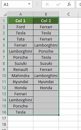
3.1. Scenario 1: Comparing Two Columns Row-by-Row
To compare two columns row-by-row, use the following formulas:
=IF(A2=B2, "match", " ")=IF(A2<>B2, "no match", " ")=IF(A2=B2, "match", "no match")
If you need the results to be case-sensitive, then use the following formulas:
=IF(EXACT(A2, B2), "Match", " ")=IF(EXACT(A2, B2), "Match," "No match")
3.2. Scenario 2: Comparing Multiple Columns for Row Matches
If you need to compare and find the differences and similarities between more than two columns, then use the following formulas:
=IF(AND(A2=B2, A2=C2), "Complete match", " ")=IF(COUNTIF($A2:$E2, $A2)=4, "Complete match," "), where 4 is the number of columns you are comparing
If you want to compare columns with any two or more cells with the same values in the same row, then you might use the following formulas:
=IF(OR(A2=B2, B2=C2, A2=C2), "Match", "")=IF(COUNTIF(B2:D2,A2)+COUNTIF(C2:D2,B2)+(C2=D2)=0,"Unique","Match")
3.3. Scenario 3: Compare Two Columns for Matches and Differences
To compare two datasets, to find the unique values present in column A and not in column B one can use any of the formulas for finding the match and differences:
=IF(COUNTIF($B:$B, $A2)=0, "Not present in B", "")=IF(ISERROR(MATCH($A2,$B$2:$B$10,0)),"No present in B","")
You can use a single formula to get the result for matches and unique values:
=IF(COUNTIF($B:$B, $A2)=0, "No Present in B", "Present in B")
3.4. Scenario 4: Compare Two Lists and Pull Matching Data
To compare two lists and find the matching data, you can use the VLOOKUP function. You can also use the INDEX MATCH formula. You can use the following formulas for this scenario:
=VLOOKUP(D2, $A$2:$B$6, 2, FALSE)=INDEX($B$2:$B$6, MATCH($D2, $A$2:$A$6, 0))=XLOOKUP(D2, $A$2:$A$6, $B$2:$B$6)
A2, B2 and D2 are the first cells of three columns. 2 is the number of columns compared.
3.5. Scenario 5: Highlight Row Matches and Differences
You can create a conditional formatting formula that can highlight the rows that include identical values in all the columns. You can use the following formula for the desired result:
=AND($A2=$B2, $A2=$C2)
or
=COUNTIF($A2:$C2, $A2)=3
3 is the number of columns and A2, B2 and C2 are the top-most cells, to compare.
You can also use the following steps to find and highlight the matches and differences in Excel:
- Select the columns with the dataset you want to compare.
- Go to the editing group section on the Home tab, click the “Find and Select” drop-down, and choose “Go To Special.” Select Row Differences and click OK.
- The cells having different values than the cells compared in each row will be colored. To change the color click the Fill Color icon on and choose the color of your choice.
4. Common Challenges and Solutions
While comparing rows in Excel, you might encounter some common challenges. Here’s how to address them:
- Inconsistent Data: Ensure data is consistent by trimming extra spaces, standardizing date formats, and correcting typos.
- Case Sensitivity: Use the EXACT function to perform case-sensitive comparisons, or convert all data to the same case using UPPER or LOWER functions.
- Large Datasets: Use Power Query or VBA scripting for better performance and efficiency when dealing with large datasets.
- Complex Criteria: Break down complex comparison criteria into smaller, manageable steps using helper columns and multiple formulas.
5. Best Practices for Accurate Comparisons
To ensure accurate comparisons, follow these best practices:
- Data Validation: Implement data validation rules to prevent inconsistent data entry.
- Regular Audits: Conduct regular data audits to identify and correct errors and inconsistencies.
- Documentation: Document your comparison methods and criteria to ensure consistency and reproducibility.
- Testing: Test your formulas and scripts thoroughly before applying them to your entire dataset.
6. Real-World Applications
Comparing rows in Excel has numerous real-world applications across various industries:
- Finance: Identifying duplicate transactions for fraud detection.
- Healthcare: Ensuring accurate patient records and preventing duplicate entries.
- Retail: Managing product catalogs and preventing duplicate listings.
- Education: Tracking student enrollment and identifying duplicate registrations.
- Manufacturing: Monitoring inventory levels and preventing duplicate orders.
7. Advanced Tips and Tricks
Here are some advanced tips and tricks to enhance your row comparison skills:
- Using Array Formulas: Array formulas can perform complex comparisons across multiple rows and columns.
- Combining Multiple Functions: Combine multiple Excel functions to create powerful comparison formulas.
- Creating Custom Functions: Create custom functions using VBA to automate repetitive comparison tasks.
- Integrating with External Data Sources: Use Power Query to import data from external sources and compare it with your Excel data.
8. How COMPARE.EDU.VN Can Help
COMPARE.EDU.VN offers a wide range of resources and tools to help you compare rows in Excel effectively. Our platform provides detailed tutorials, practical examples, and customizable templates to streamline your data management tasks. Whether you’re a beginner or an experienced Excel user, COMPARE.EDU.VN can help you enhance your row comparison skills and ensure data accuracy. With us, you can improve data quality and streamline your data management.
Are you struggling to compare data across different platforms? COMPARE.EDU.VN offers comprehensive comparisons and solutions to help you make informed decisions.
9. Case Studies
Let’s explore a couple of case studies to illustrate the effectiveness of these methods:
9.1. Case Study 1: Finance
A financial institution needed to identify duplicate transactions in their database to detect potential fraud. By using conditional formatting and the COUNTIF function, they were able to quickly flag duplicate transactions based on matching amounts and dates. This allowed them to investigate and prevent fraudulent activities, saving the company significant financial losses.
9.2. Case Study 2: Healthcare
A healthcare provider needed to ensure accurate patient records by identifying duplicate entries. By using the Advanced Filter and Power Query, they were able to extract unique patient entries based on matching names and birthdates. This helped them maintain a clean and accurate patient database, improving the quality of care and reducing the risk of medical errors.
10. FAQs
10.1. How to compare two rows in Excel?
Use formulas like =IF(A1=A2, "Match", "No Match") or conditional formatting to highlight differences.
10.2. Is it possible to compare two rows in Excel using the Index-Match function?
Yes, you can use INDEX-MATCH to compare values in different rows based on specific criteria.
10.3. How to compare multiple rows in Excel?
Use formulas like =IF(AND(A1=A2, B1=B2), "Match", "No Match") or Power Query for more complex comparisons.
10.4. How do you compare two lists in Excel for matches?
Use VLOOKUP, INDEX-MATCH, or conditional formatting to find matching entries.
10.5. How can I compare rows and highlight the first occurrence of a mismatch?
Use conditional formatting with a formula like =A1<>A2 to highlight the first mismatch.
10.6. How do I compare rows for duplicates only?
Use the COUNTIF function to identify rows that appear more than once.
10.7. Can I compare rows and count the number of matches or differences?
Yes, use SUMPRODUCT or COUNTIF to count matches and differences between rows.
11. Conclusion
Comparing rows in Excel is a crucial skill for anyone working with data. By mastering the methods and techniques outlined in this article, you can efficiently identify duplicate entries, ensure data accuracy, and make informed decisions. Whether you’re using conditional formatting, the COUNTIF function, Advanced Filter, Power Query, or VBA scripting, COMPARE.EDU.VN is here to support you every step of the way.
Ready to take your data analysis skills to the next level? Visit COMPARE.EDU.VN today to explore our comprehensive tutorials, practical examples, and customizable templates. Start comparing rows in Excel like a pro and unlock the full potential of your data. We provide accurate and easy to understand comparisons.
Address: 333 Comparison Plaza, Choice City, CA 90210, United States
WhatsApp: +1 (626) 555-9090
Website: compare.edu.vn