In order to accurately assess the disparities between two separate groups, understanding How To Compare Proportions Between Two Groups is essential, and COMPARE.EDU.VN helps simplify this complex task. This article will help you understand the statistical methods used to determine whether observed differences are statistically significant or just happened by chance, offering you an objective approach to comparative data analysis. Explore reliable comparative insights and make smarter decisions with detailed comparisons from COMPARE.EDU.VN, powered by in-depth data analysis and user-friendly presentation. You’ll gain a strong grasp of hypothesis testing, confidence intervals, and comparing data sets by the end of this guide, which will enable you to confidently evaluate and draw insightful conclusions.
1. Understanding the Basics of Comparing Proportions
Before diving into the specifics of comparing proportions, it’s crucial to understand the underlying concepts. Comparing proportions involves assessing whether the difference between two sample proportions is statistically significant, meaning it’s unlikely to have occurred by random chance. This process is fundamental in various fields, including medicine, marketing, and social sciences, where comparing the success rates or prevalence of certain characteristics between different groups is common.
1.1. What is a Proportion?
A proportion represents the fraction of a population that possesses a specific characteristic. It’s calculated by dividing the number of individuals with the characteristic by the total number of individuals in the group. For example, if you survey 500 people and find that 350 prefer a certain brand, the sample proportion is 350/500 = 0.7, or 70%. This basic calculation is the foundation for more advanced statistical comparisons.
1.2. Why Compare Proportions?
Comparing proportions is essential because it allows you to determine if observed differences between groups are meaningful or simply due to random variation. For instance, a marketing team might want to know if a higher percentage of customers from one demographic group respond positively to an advertising campaign compared to another group. Similarly, in clinical trials, researchers compare the proportion of patients experiencing positive outcomes in a treatment group versus a control group.
1.3. Key Concepts in Hypothesis Testing
Hypothesis testing is the cornerstone of comparing proportions. Here are the key concepts:
- Null Hypothesis (H₀): Assumes there is no difference between the population proportions being compared. For example, H₀: p₁ = p₂, where p₁ and p₂ are the population proportions of the two groups.
- Alternative Hypothesis (H₁ or Ha): States that there is a difference between the population proportions. This can be directional (e.g., p₁ > p₂ or p₁ < p₂) or non-directional (e.g., p₁ ≠ p₂).
- Significance Level (α): The probability of rejecting the null hypothesis when it is true. Common values are 0.05 (5%) and 0.01 (1%).
- P-value: The probability of observing a test statistic as extreme as, or more extreme than, the one computed from the sample data, assuming the null hypothesis is true.
- Test Statistic: A standardized value calculated from the sample data that is used to determine the p-value. For comparing proportions, the z-score is commonly used.
2. Conditions for Conducting a Two-Proportion Z-Test
Before you can confidently compare proportions between two groups using a z-test, you need to ensure that certain conditions are met. These conditions guarantee that the test results are reliable and valid.
2.1. Independence
The samples from the two groups must be independent of each other. This means that the data from one group should not influence the data from the other group. Random sampling helps ensure independence, where each member of the population has an equal chance of being selected.
2.2. Random Sampling
Both samples should be obtained through simple random sampling. This ensures that the samples are representative of the populations they are drawn from, minimizing bias and increasing the generalizability of the findings.
2.3. Sample Size
The sample sizes should be large enough to ensure that the sampling distribution of the sample proportions is approximately normal. A common rule of thumb is to verify that:
- n₁p₁ ≥ 5 and n₁(1 – p₁) ≥ 5 for the first sample.
- n₂p₂ ≥ 5 and n₂(1 – p₂) ≥ 5 for the second sample.
Here, n₁ and n₂ are the sample sizes, and p₁ and p₂ are the sample proportions. Meeting these conditions ensures that the normal approximation is appropriate.
2.4. Population Size
The population size for both groups must be large relative to the sample size. A common guideline is that each population should be at least 10 to 20 times larger than its corresponding sample size. This condition helps prevent over-sampling, which can lead to incorrect results.
3. The Two-Proportion Z-Test: A Step-by-Step Guide
The two-proportion z-test is a statistical method used to determine if there is a significant difference between the proportions of two independent groups. Here’s a step-by-step guide on how to conduct this test.
3.1. State the Null and Alternative Hypotheses
Start by defining the null and alternative hypotheses. The null hypothesis (H₀) typically states that there is no difference between the two population proportions (p₁ = p₂). The alternative hypothesis (H₁) can be directional or non-directional:
- Non-directional: H₁: p₁ ≠ p₂ (the proportions are different).
- Right-tailed: H₁: p₁ > p₂ (the proportion of group 1 is greater than group 2).
- Left-tailed: H₁: p₁ < p₂ (the proportion of group 1 is less than group 2).
3.2. Calculate the Sample Proportions
Calculate the sample proportions for both groups:
- (hat{p}_1 = frac{x_1}{n_1}), where x₁ is the number of successes in sample 1, and n₁ is the sample size of group 1.
- (hat{p}_2 = frac{x_2}{n_2}), where x₂ is the number of successes in sample 2, and n₂ is the sample size of group 2.
3.3. Compute the Pooled Proportion
The pooled proportion (pc) is a weighted average of the two sample proportions, assuming the null hypothesis is true (i.e., the population proportions are equal):
[p_{c} = frac{x_{1} + x_{2}}{n_{1} + n_{2}}]
This pooled proportion is used to estimate the standard error of the difference between the two proportions.
3.4. Calculate the Test Statistic (Z-score)
The z-score is calculated using the following formula:
[z = frac{(hat{p}_{1} – hat{p}_{2})}{sqrt{p_{c}(1 – p_{c})left(frac{1}{n_{1}} + frac{1}{n_{2}}right)}}]
This z-score measures how many standard errors the observed difference between the sample proportions is from zero, assuming the null hypothesis is true.
3.5. Determine the P-value
The p-value is the probability of observing a test statistic as extreme as, or more extreme than, the one calculated, assuming the null hypothesis is true. You can find the p-value using a standard normal distribution table or a statistical calculator.
- For a non-directional (two-tailed) test, the p-value is 2 * P(Z > |z|).
- For a right-tailed test, the p-value is P(Z > z).
- For a left-tailed test, the p-value is P(Z < z).
3.6. Make a Decision
Compare the p-value to the significance level (α). If the p-value is less than or equal to α, reject the null hypothesis. This indicates that there is a statistically significant difference between the two population proportions. If the p-value is greater than α, fail to reject the null hypothesis, meaning there is not enough evidence to conclude that the proportions are different.
3.7. Draw a Conclusion
Interpret the results in the context of the problem. If you reject the null hypothesis, state that there is a significant difference between the proportions, and describe the direction of the difference if the alternative hypothesis was directional. If you fail to reject the null hypothesis, state that there is not enough evidence to conclude that the proportions are different.
4. Confidence Intervals for the Difference Between Two Proportions
In addition to hypothesis testing, constructing a confidence interval for the difference between two proportions provides a range of plausible values for the true difference in population proportions.
4.1. Formula for the Confidence Interval
The confidence interval for the difference between two population proportions is calculated as follows:
[(hat{p}_{1} – hat{p}_{2}) pm z_{frac{alpha}{2}}sqrt{frac{hat{p}_{1}(1 – hat{p}_{1})}{n_{1}} + frac{hat{p}_{2}(1 – hat{p}_{2})}{n_{2}}}]
Here:
- (hat{p}_{1}) and (hat{p}_{2}) are the sample proportions.
- n₁ and n₂ are the sample sizes.
- (z_{frac{alpha}{2}}) is the z-score corresponding to the desired confidence level (e.g., for a 95% confidence interval, (z_{frac{alpha}{2}}) = 1.96).
4.2. Interpreting the Confidence Interval
The confidence interval provides a range within which the true difference between the population proportions is likely to fall. For example, a 95% confidence interval means that if you were to take many samples and construct confidence intervals for each sample, 95% of those intervals would contain the true difference between the population proportions.
- If the confidence interval includes zero, it suggests that there may not be a significant difference between the two population proportions.
- If the confidence interval does not include zero, it suggests that there is a significant difference between the two population proportions. The sign of the interval indicates the direction of the difference.
4.3. Practical Example
Suppose you want to estimate the difference in customer satisfaction between two brands, A and B. You survey 200 customers of brand A and find that 150 are satisfied. You survey 250 customers of brand B and find that 180 are satisfied. The sample proportions are (hat{p}_{A} = frac{150}{200} = 0.75) and (hat{p}_{B} = frac{180}{250} = 0.72).
To construct a 95% confidence interval, you use the formula:
[(0.75 – 0.72) pm 1.96sqrt{frac{0.75(1 – 0.75)}{200} + frac{0.72(1 – 0.72)}{250}}]
[0.03 pm 1.96sqrt{frac{0.1875}{200} + frac{0.2016}{250}}]
[0.03 pm 1.96sqrt{0.0009375 + 0.0008064}]
[0.03 pm 1.96sqrt{0.0017439}]
[0.03 pm 1.96(0.04176)]
[0.03 pm 0.0818]
The 95% confidence interval is [-0.0518, 0.1118]. Since the interval includes zero, you cannot conclude that there is a significant difference in customer satisfaction between the two brands at the 95% confidence level.
5. Practical Examples and Case Studies
To further illustrate how to compare proportions between two groups, let’s examine a few practical examples and case studies.
5.1. Example 1: Medical Research
A pharmaceutical company is testing a new drug to treat a specific condition. In a clinical trial, 300 patients are given the drug, and 210 show improvement. In a control group of 250 patients receiving a placebo, 150 show improvement. The goal is to determine if the drug is more effective than the placebo.
- Group 1 (Drug): n₁ = 300, x₁ = 210, (hat{p}_{1} = frac{210}{300} = 0.7)
- Group 2 (Placebo): n₂ = 250, x₂ = 150, (hat{p}_{2} = frac{150}{250} = 0.6)
1. State the Hypotheses:
- H₀: p₁ = p₂ (there is no difference in improvement rates between the drug and placebo).
- H₁: p₁ > p₂ (the drug is more effective than the placebo).
2. Calculate the Pooled Proportion:
[p_{c} = frac{210 + 150}{300 + 250} = frac{360}{550} = 0.6545]
3. Calculate the Test Statistic:
[z = frac{(0.7 – 0.6)}{sqrt{0.6545(1 – 0.6545)left(frac{1}{300} + frac{1}{250}right)}}]
[z = frac{0.1}{sqrt{0.6545(0.3455)left(0.00333 + 0.004right)}}]
[z = frac{0.1}{sqrt{0.2259left(0.00733right)}}]
[z = frac{0.1}{sqrt{0.001656}}]
[z = frac{0.1}{0.0407}]
[z = 2.457]
4. Determine the P-value:
For a right-tailed test, P(Z > 2.457) ≈ 0.007.
5. Make a Decision:
If α = 0.05, since 0.007 < 0.05, reject the null hypothesis.
6. Draw a Conclusion:
At the 5% significance level, there is sufficient evidence to conclude that the drug is more effective than the placebo in improving the condition.
5.2. Example 2: Marketing Campaign Analysis
A marketing team runs two different advertising campaigns to promote a product. Campaign A is shown to 400 people, and 60 make a purchase. Campaign B is shown to 500 people, and 70 make a purchase. The team wants to know if there is a significant difference in the effectiveness of the two campaigns.
- Group 1 (Campaign A): n₁ = 400, x₁ = 60, (hat{p}_{1} = frac{60}{400} = 0.15)
- Group 2 (Campaign B): n₂ = 500, x₂ = 70, (hat{p}_{2} = frac{70}{500} = 0.14)
1. State the Hypotheses:
- H₀: p₁ = p₂ (there is no difference in effectiveness between the two campaigns).
- H₁: p₁ ≠ p₂ (the campaigns have different effectiveness).
2. Calculate the Pooled Proportion:
[p_{c} = frac{60 + 70}{400 + 500} = frac{130}{900} = 0.1444]
3. Calculate the Test Statistic:
[z = frac{(0.15 – 0.14)}{sqrt{0.1444(1 – 0.1444)left(frac{1}{400} + frac{1}{500}right)}}]
[z = frac{0.01}{sqrt{0.1444(0.8556)left(0.0025 + 0.002right)}}]
[z = frac{0.01}{sqrt{0.1235left(0.0045right)}}]
[z = frac{0.01}{sqrt{0.00055575}}]
[z = frac{0.01}{0.02357}]
[z = 0.424]
4. Determine the P-value:
For a two-tailed test, P(Z > |0.424|) = 2 P(Z > 0.424) ≈ 2 0.3357 = 0.6714.
5. Make a Decision:
If α = 0.05, since 0.6714 > 0.05, fail to reject the null hypothesis.
6. Draw a Conclusion:
At the 5% significance level, there is not enough evidence to conclude that the two marketing campaigns have different effectiveness.
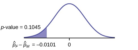 A curved line graph displaying a normal distribution with the mean at zero. Shaded areas under the curve's tail, one left and one right, indicate a p-value of 0.1045.
5.3. Case Study: Educational Program Evaluation
An educational researcher is evaluating the effectiveness of a new teaching method compared to the traditional method. They randomly assign 200 students to the new method (Group A) and 250 students to the traditional method (Group B). At the end of the semester, 160 students in Group A and 180 students in Group B pass the final exam. The researcher wants to determine if the new method leads to a higher proportion of students passing the exam.
- Group A (New Method): n₁ = 200, x₁ = 160, (hat{p}_{1} = frac{160}{200} = 0.8)
- Group B (Traditional Method): n₂ = 250, x₂ = 180, (hat{p}_{2} = frac{180}{250} = 0.72)
1. State the Hypotheses:
- H₀: p₁ = p₂ (there is no difference in pass rates between the new and traditional methods).
- H₁: p₁ > p₂ (the new method leads to a higher pass rate).
2. Calculate the Pooled Proportion:
[p_{c} = frac{160 + 180}{200 + 250} = frac{340}{450} = 0.7556]
3. Calculate the Test Statistic:
[z = frac{(0.8 – 0.72)}{sqrt{0.7556(1 – 0.7556)left(frac{1}{200} + frac{1}{250}right)}}]
[z = frac{0.08}{sqrt{0.7556(0.2444)left(0.005 + 0.004right)}}]
[z = frac{0.08}{sqrt{0.1847left(0.009right)}}]
[z = frac{0.08}{sqrt{0.0016623}}]
[z = frac{0.08}{0.04077}]
[z = 1.962]
4. Determine the P-value:
For a right-tailed test, P(Z > 1.962) ≈ 0.025.
5. Make a Decision:
If α = 0.05, since 0.025 < 0.05, reject the null hypothesis.
6. Draw a Conclusion:
At the 5% significance level, there is sufficient evidence to conclude that the new teaching method leads to a higher proportion of students passing the final exam compared to the traditional method.
6. Common Pitfalls and How to Avoid Them
When comparing proportions between two groups, several common pitfalls can lead to incorrect conclusions. Here’s how to avoid them:
6.1. Ignoring the Conditions for the Z-Test
Failing to verify the conditions for the z-test (independence, random sampling, sample size, and population size) can lead to unreliable results.
Solution: Always check these conditions before performing the z-test. If the conditions are not met, consider using alternative methods or collecting more data.
6.2. Misinterpreting the P-value
The p-value is the probability of observing the data (or more extreme data) if the null hypothesis is true, not the probability that the null hypothesis is true.
Solution: Understand that the p-value only provides evidence against the null hypothesis. A small p-value suggests that the observed data is unlikely if the null hypothesis is true, leading you to reject it.
6.3. Failing to Consider Practical Significance
Statistical significance does not always imply practical significance. A statistically significant difference may be too small to be meaningful in a real-world context.
Solution: Consider the effect size (e.g., the difference between the sample proportions) and its practical implications, in addition to statistical significance.
6.4. Making Causation Claims Based on Observational Data
Observational studies can show associations between variables but cannot establish causation.
Solution: Be cautious about making causal claims unless the data comes from a well-designed experiment. In observational studies, focus on describing associations and potential confounding factors.
6.5. Not Adjusting for Multiple Comparisons
When conducting multiple hypothesis tests, the probability of making at least one Type I error (rejecting a true null hypothesis) increases.
Solution: Use methods like the Bonferroni correction or the Benjamini-Hochberg procedure to adjust the significance level when performing multiple comparisons.
7. Advanced Techniques and Considerations
For more complex scenarios, there are several advanced techniques and considerations to keep in mind when comparing proportions.
7.1. Chi-Square Test
The chi-square test is another method used to compare proportions, particularly when dealing with categorical data in contingency tables.
7.2. Fisher’s Exact Test
When sample sizes are small, Fisher’s exact test provides a more accurate alternative to the z-test or chi-square test.
7.3. Bayesian Methods
Bayesian methods offer a flexible framework for comparing proportions, allowing you to incorporate prior beliefs and update them based on the observed data.
7.4. Power Analysis
Power analysis helps determine the sample size needed to detect a statistically significant difference between proportions, given a specific significance level and desired power (the probability of correctly rejecting a false null hypothesis).
7.5. Confounding Variables
When comparing proportions between two groups, it’s important to consider potential confounding variables that could influence the results.
8. Tools and Resources for Comparing Proportions
Several tools and resources can assist you in comparing proportions between two groups, making the process more efficient and accurate.
8.1. Statistical Software Packages
- R: A free, open-source statistical computing environment.
- Python (with libraries like SciPy and Statsmodels): A versatile programming language with powerful statistical analysis capabilities.
- SPSS: A widely used statistical software package with a user-friendly interface.
- SAS: A comprehensive statistical software suite often used in business and research settings.
8.2. Online Calculators
Numerous online calculators can quickly perform two-proportion z-tests and calculate confidence intervals. These calculators are useful for quick checks and simple analyses.
8.3. Spreadsheets
Spreadsheet programs like Microsoft Excel and Google Sheets can perform basic statistical calculations and are useful for organizing and visualizing data.
8.4. Educational Resources
- Statistics Textbooks: Comprehensive guides covering statistical concepts and methods.
- Online Courses: Platforms like Coursera, edX, and Khan Academy offer courses on statistics and data analysis.
- Statistical Journals: Publications like the Journal of the American Statistical Association and Biometrics provide cutting-edge research on statistical methods.
9. Future Trends in Statistical Comparison
The field of statistical comparison is continually evolving, driven by advancements in technology and increasing data availability. Here are some future trends to watch:
9.1. Machine Learning Integration
Machine learning algorithms are being increasingly used to analyze complex datasets and identify subtle differences between groups that traditional statistical methods might miss.
9.2. Big Data Analytics
As data volumes grow, new techniques are being developed to efficiently compare proportions in large datasets, addressing computational challenges and ensuring accurate results.
9.3. Enhanced Visualization
Interactive and dynamic visualizations are becoming more common, allowing users to explore differences between groups in an intuitive and engaging way.
9.4. Improved Accessibility
Efforts are underway to make statistical tools and methods more accessible to non-statisticians, enabling a wider audience to conduct meaningful comparisons and make data-driven decisions.
10. Conclusion: Making Informed Decisions with COMPARE.EDU.VN
Understanding how to compare proportions between two groups is essential for anyone who needs to make data-driven decisions. This guide has provided a comprehensive overview of the key concepts, steps, and considerations involved in this process. By following the guidelines outlined in this article, you can confidently evaluate and draw insightful conclusions from comparative data.
Remember, accurate statistical comparison requires careful attention to detail and a thorough understanding of the underlying assumptions. By leveraging the tools and resources available, you can ensure that your analyses are robust and reliable.
For more detailed comparisons and help making informed decisions, visit COMPARE.EDU.VN. Our platform offers detailed and objective comparisons across a wide range of products, services, and ideas, empowering you to make the best choices for your needs.
Visit COMPARE.EDU.VN today to explore our comprehensive comparisons and make your next decision with confidence.
Address: 333 Comparison Plaza, Choice City, CA 90210, United States.
Whatsapp: +1 (626) 555-9090.
Website: COMPARE.EDU.VN
FAQ: Comparing Proportions Between Two Groups
1. What is the purpose of comparing proportions between two groups?
Comparing proportions helps determine if observed differences between groups are statistically significant or due to random chance. This is vital in fields like medicine, marketing, and social sciences.
2. What conditions must be met to conduct a two-proportion z-test?
The samples must be independent, randomly selected, large enough (n₁p₁ ≥ 5 and n₁(1 – p₁) ≥ 5), and the population size must be large relative to the sample size.
3. How do you calculate the pooled proportion?
The pooled proportion (pc) is calculated as [p_{c} = frac{x_{1} + x_{2}}{n_{1} + n_{2}}], where x₁ and x₂ are the number of successes, and n₁ and n₂ are the sample sizes.
4. What does the p-value tell you in a two-proportion z-test?
The p-value is the probability of observing a test statistic as extreme as, or more extreme than, the one calculated, assuming the null hypothesis is true.
5. How do you interpret a confidence interval for the difference between two proportions?
If the interval includes zero, there may not be a significant difference. If it does not include zero, there is a significant difference, with the sign indicating the direction.
6. What are some common pitfalls to avoid when comparing proportions?
Common pitfalls include ignoring test conditions, misinterpreting the p-value, failing to consider practical significance, making causation claims based on observational data, and not adjusting for multiple comparisons.
7. When should you use Fisher’s exact test instead of a z-test?
Fisher’s exact test should be used when sample sizes are small, as it provides a more accurate alternative.
8. How can machine learning be used in statistical comparison?
Machine learning algorithms can analyze complex datasets and identify subtle differences between groups that traditional statistical methods might miss.
9. What is power analysis, and why is it important?
Power analysis helps determine the sample size needed to detect a statistically significant difference, given a specific significance level and desired power.
10. Where can you find reliable and objective comparisons to aid decision-making?
Visit compare.edu.vn for detailed and objective comparisons across a wide range of products, services, and ideas.