How To Compare One Column With Multiple Columns In Excel

Comparing one column with multiple columns in Excel can be a complex task, but COMPARE.EDU.VN offers solutions. This guide provides methods and formulas to efficiently compare data, identify matches, and highlight differences. Understand data comparison in Excel.

1. Understanding the Need for Column Comparison in Excel

In Excel, comparing columns is essential for various data analysis tasks. Whether you’re verifying data integrity, identifying discrepancies, or merging datasets, effective column comparison techniques are invaluable. This article will guide you through various methods to compare one column with multiple columns in Excel, ensuring you can tackle any data comparison challenge with ease.

1.1. Why Compare Columns in Excel?

Comparing columns in Excel serves several critical purposes:

• Data Validation: Ensuring data accuracy and consistency across different sources.
• Identifying Discrepancies: Spotting differences in data entries, which is crucial for error detection.
• Merging Datasets: Combining data from multiple sources while identifying and resolving conflicts.
• Duplicate Detection: Finding and removing duplicate entries within a dataset.
• Trend Analysis: Comparing data over different periods to identify trends and patterns.

1.2. Common Scenarios for Column Comparison

Here are some common scenarios where column comparison in Excel is beneficial:

• Financial Audits: Comparing financial records from different departments to ensure accuracy.
• Inventory Management: Matching inventory lists with sales records to track stock levels.
• Customer Relationship Management (CRM): Validating customer data across different CRM systems.
• Research Analysis: Comparing data from multiple surveys or experiments to identify significant results.
• Human Resources: Verifying employee data across different HR systems.

2. Basic Techniques for Comparing Columns in Excel

Excel offers several basic techniques for comparing columns, which are useful for simple comparisons and identifying obvious differences.

2.1. Using Conditional Formatting

Conditional formatting allows you to highlight cells based on specific criteria. This method is useful for visually identifying differences between columns.

Steps:

1. Select the Columns: Choose the columns you want to compare.
2. Go to Conditional Formatting: On the “Home” tab, click on “Conditional Formatting.”
3. Choose Highlight Cells Rule: Select “Highlight Cells Rules” and then “Duplicate Values.”
4. Customize the Rule: Choose “Unique” in the dropdown to highlight unique values in the selected columns.
5. Apply Formatting: Select the formatting style you want to apply to the unique values (e.g., fill color, font color).
6. Click OK: The unique values will be highlighted in the selected columns.

This technique helps you quickly identify entries that are present in one column but not in the others.

2.2. Employing Simple Formulas

Simple formulas can be used to compare corresponding cells in different columns. This method is suitable for comparing data row by row.

Example:

If you want to compare column A with column B, you can use the following formula in column C:

=IF(A1=B1, "Match", "Mismatch")

Steps:

1. Enter the Formula: In cell C1, enter the formula =IF(A1=B1, "Match", "Mismatch").
2. Copy the Formula: Drag the fill handle (the small square at the bottom-right of the cell) down to apply the formula to all rows.
3. Review the Results: Column C will now display “Match” for rows where the values in column A and column B are the same, and “Mismatch” for rows where they are different.

This method is straightforward and provides a clear indication of whether the values in each row match.

2.3. Using the EXACT Function

The EXACT function compares two text strings and returns TRUE if they are exactly the same, including case. This function is useful for case-sensitive comparisons.

Example:

To compare column A with column B using the EXACT function, use the following formula in column C:

=EXACT(A1, B1)

Steps:

1. Enter the Formula: In cell C1, enter the formula =EXACT(A1, B1).
2. Copy the Formula: Drag the fill handle down to apply the formula to all rows.
3. Review the Results: Column C will display TRUE if the text in column A and column B are exactly the same (including case), and FALSE if they are different.

This technique is particularly useful when case sensitivity is important in your data comparison.

3. Advanced Techniques for Comparing Columns in Excel

For more complex comparisons, Excel offers advanced techniques that can handle large datasets and intricate comparison criteria.

3.1. Using the VLOOKUP Function

The VLOOKUP function is used to find a value in one column and return a corresponding value from another column. It can be used to check if a value from one column exists in another column.

Example:

To check if the values in column A exist in column B, use the following formula in column C:

=IF(ISNA(VLOOKUP(A1, B:B, 1, FALSE)), "Not Found", "Found")

Steps:

1. Enter the Formula: In cell C1, enter the formula =IF(ISNA(VLOOKUP(A1, B:B, 1, FALSE)), "Not Found", "Found").
2. Copy the Formula: Drag the fill handle down to apply the formula to all rows.
3. Review the Results: Column C will display “Found” if the value from column A exists in column B, and “Not Found” if it does not.

This method is useful for identifying missing values or verifying the presence of specific entries across multiple columns.

3.2. Combining INDEX and MATCH Functions

The INDEX and MATCH functions can be combined to perform more flexible lookups than VLOOKUP. This combination allows you to look up values based on multiple criteria and return corresponding values from different columns.

Example:

To find the corresponding value in column C for a value in column A that matches a value in column B, use the following formula:

=INDEX(C:C, MATCH(A1, B:B, 0))

Steps:

1. Enter the Formula: In cell D1 (or any other column), enter the formula =INDEX(C:C, MATCH(A1, B:B, 0)).
2. Copy the Formula: Drag the fill handle down to apply the formula to all rows.
3. Review the Results: Column D will display the corresponding value from column C for each value in column A that matches a value in column B. If there is no match, it will return an error.

This technique is powerful for performing complex lookups and retrieving data based on multiple conditions.

3.3. Utilizing Array Formulas

Array formulas allow you to perform calculations on multiple values at once. They are useful for comparing entire columns or ranges of data.

Example:

To count the number of matches between column A and column B, you can use the following array formula:

=SUM(IF(A1:A100=B1:B100, 1, 0))

Steps:

1. Enter the Formula: In a cell, enter the formula =SUM(IF(A1:A100=B1:B100, 1, 0)).
2. Enter as Array Formula: Press Ctrl + Shift + Enter to enter the formula as an array formula. Excel will automatically add curly braces {} around the formula.
3. Review the Result: The cell will display the number of matches between the values in column A and column B.

Array formulas are versatile and can be used for various complex comparisons.

3.4. Using the COUNTIF and COUNTIFS Functions

The COUNTIF and COUNTIFS functions are used to count the number of cells that meet a specific criterion. These functions are useful for identifying duplicate or unique values across columns.

Example:

To count how many times a value from column A appears in column B, use the following formula in column C:

=COUNTIF(B:B, A1)

Steps:

1. Enter the Formula: In cell C1, enter the formula =COUNTIF(B:B, A1).
2. Copy the Formula: Drag the fill handle down to apply the formula to all rows.
3. Review the Results: Column C will display the number of times each value from column A appears in column B.

For multiple criteria, you can use the COUNTIFS function. For example, to count the number of rows where column A equals a specific value and column B equals another value, use the following formula:

=COUNTIFS(A:A, "value1", B:B, "value2")

These functions are valuable for analyzing data and identifying patterns based on specific criteria.

4. Comparing One Column with Multiple Columns

When you need to compare one column against multiple columns, you can combine the techniques mentioned above to achieve the desired results.

4.1. Using Multiple VLOOKUP Functions

You can use multiple VLOOKUP functions to check if a value from one column exists in multiple other columns.

Example:

To check if the values in column A exist in columns B, C, and D, use the following formula in column E:

=IF(OR(NOT(ISNA(VLOOKUP(A1, B:B, 1, FALSE))), NOT(ISNA(VLOOKUP(A1, C:C, 1, FALSE))), NOT(ISNA(VLOOKUP(A1, D:D, 1, FALSE)))), "Found", "Not Found")

Steps:

1. Enter the Formula: In cell E1, enter the formula =IF(OR(NOT(ISNA(VLOOKUP(A1, B:B, 1, FALSE))), NOT(ISNA(VLOOKUP(A1, C:C, 1, FALSE))), NOT(ISNA(VLOOKUP(A1, D:D, 1, FALSE)))), "Found", "Not Found").
2. Copy the Formula: Drag the fill handle down to apply the formula to all rows.
3. Review the Results: Column E will display “Found” if the value from column A exists in any of the columns B, C, or D, and “Not Found” if it does not exist in any of them.

This method is useful for identifying whether a value is present in any of the multiple columns being compared.

4.2. Combining COUNTIF with OR Function

You can combine the COUNTIF function with the OR function to check if a value from one column appears in any of the multiple columns.

Example:

To check if the values in column A appear in any of the columns B, C, and D, use the following formula in column E:

=IF(OR(COUNTIF(B:B, A1)>0, COUNTIF(C:C, A1)>0, COUNTIF(D:D, A1)>0), "Found", "Not Found")

Steps:

1. Enter the Formula: In cell E1, enter the formula =IF(OR(COUNTIF(B:B, A1)>0, COUNTIF(C:C, A1)>0, COUNTIF(D:D, A1)>0), "Found", "Not Found").
2. Copy the Formula: Drag the fill handle down to apply the formula to all rows.
3. Review the Results: Column E will display “Found” if the value from column A appears in any of the columns B, C, or D, and “Not Found” if it does not appear in any of them.

This technique is effective for identifying the presence of a value across multiple columns using the COUNTIF function.

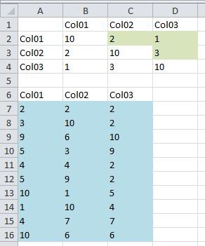
4.3. Creating a Comparison Matrix

For a more structured approach, you can create a comparison matrix to compare one column against multiple columns. This involves creating a table that shows the matches between the values in each column.

Steps:

1. Set Up the Matrix: Create a table with the column headers of the columns you want to compare in both the rows and columns.
2. Enter the Formula: In each cell of the matrix, enter a formula that compares the corresponding columns. For example, to compare column A with column B, you can use the formula =SUM(IF(A1:A100=B1:B100, 1, 0)) as an array formula.
3. Apply the Formula: Apply the formula to all cells in the matrix.
4. Review the Results: The matrix will show the number of matches between each pair of columns.

This method provides a clear overview of the relationships between the values in different columns.

4.4. Using Helper Columns

Helper columns can simplify the comparison process by breaking down the comparison into smaller, more manageable steps.

Example:

To compare column A with columns B, C, and D, you can create helper columns that indicate whether the value from column A exists in each of the other columns.

Steps:

1. Create Helper Columns: Create three new columns (e.g., E, F, and G) next to column D.
2. Enter the Formulas:
   • In cell E1, enter the formula =IF(ISNA(VLOOKUP(A1, B:B, 1, FALSE)), 0, 1).
   • In cell F1, enter the formula =IF(ISNA(VLOOKUP(A1, C:C, 1, FALSE)), 0, 1).
   • In cell G1, enter the formula =IF(ISNA(VLOOKUP(A1, D:D, 1, FALSE)), 0, 1).
3. Copy the Formulas: Drag the fill handle down to apply the formulas to all rows.
4. Combine the Results: In column H, enter the formula =IF(SUM(E1:G1)>0, "Found", "Not Found").
5. Review the Results: Column H will display “Found” if the value from column A exists in any of the columns B, C, or D, and “Not Found” if it does not exist in any of them.

Helper columns make it easier to understand and troubleshoot the comparison process by breaking it down into smaller steps.

5. Practical Examples of Column Comparison in Excel

To further illustrate the techniques discussed, let’s look at some practical examples of column comparison in Excel.

5.1. Comparing Customer Lists

Suppose you have two customer lists in columns A and B, and you want to identify customers who are present in both lists.

Steps:

1. Use VLOOKUP: In column C, enter the formula =IF(ISNA(VLOOKUP(A1, B:B, 1, FALSE)), "Not Found", "Found").
2. Copy the Formula: Drag the fill handle down to apply the formula to all rows.
3. Filter the Results: Filter column C to show only the “Found” values, which represent the customers who are present in both lists.

This method allows you to quickly identify common customers between the two lists.

5.2. Identifying Duplicate Product IDs

If you have a list of product IDs in column A and you want to identify any duplicates, you can use the COUNTIF function.

Steps:

1. Use COUNTIF: In column B, enter the formula =COUNTIF(A:A, A1).
2. Copy the Formula: Drag the fill handle down to apply the formula to all rows.
3. Filter the Results: Filter column B to show values greater than 1, which represent the duplicate product IDs.

This technique helps you identify and remove duplicate entries from your product list.

5.3. Validating Data Entries

Suppose you have a list of data entries in column A and you want to validate them against a master list in column B.

Steps:

1. Use VLOOKUP: In column C, enter the formula =IF(ISNA(VLOOKUP(A1, B:B, 1, FALSE)), "Invalid", "Valid").
2. Copy the Formula: Drag the fill handle down to apply the formula to all rows.
3. Filter the Results: Filter column C to show only the “Invalid” values, which represent the data entries that do not match the master list.

This method ensures that your data entries are accurate and consistent with the master list.

5.4. Comparing Sales Data Across Regions

If you have sales data for different regions in columns A, B, and C, and you want to compare the sales performance across these regions, you can use the following steps:

Steps:

1. Calculate Total Sales: In column D, calculate the total sales for each row by using the formula =SUM(A1:C1).
2. Copy the Formula: Drag the fill handle down to apply the formula to all rows.
3. Analyze the Results: Use charts and graphs to visualize the sales data and compare the performance across different regions.

This technique provides insights into the sales performance of different regions and helps you identify areas for improvement.

6. Automating Column Comparison with VBA

For more complex and repetitive tasks, you can automate the column comparison process using VBA (Visual Basic for Applications).

6.1. Writing a VBA Macro to Compare Columns

Here’s an example of a VBA macro that compares column A with column B and highlights the differences:

Sub CompareColumns()
    Dim ws As Worksheet
    Dim lastRow As Long
    Dim i As Long

    ' Set the worksheet
    Set ws = ThisWorkbook.Sheets("Sheet1") ' Change "Sheet1" to your sheet name

    ' Find the last row with data in column A
    lastRow = ws.Cells(Rows.Count, "A").End(xlUp).Row

    ' Loop through each row
    For i = 1 To lastRow
        ' Compare the values in column A and column B
        If ws.Cells(i, "A").Value <> ws.Cells(i, "B").Value Then
            ' Highlight the cell in column A if there is a difference
            ws.Cells(i, "A").Interior.Color = RGB(255, 0, 0) ' Red color
        End If
    Next i

    MsgBox "Column comparison complete!"
End Sub

Steps:

1. Open VBA Editor: Press Alt + F11 to open the VBA editor.
2. Insert a Module: Go to Insert > Module.
3. Paste the Code: Paste the VBA code into the module.
4. Modify the Code:
   • Change "Sheet1" to the name of your worksheet.
   • Adjust the column letters ("A" and "B") if you are comparing different columns.
   • Modify the highlight color (RGB(255, 0, 0)) if desired.
5. Run the Macro: Press F5 or click the “Run” button to execute the macro.

This macro will compare the values in column A and column B and highlight any differences in column A.

6.2. Creating a Custom Function for Column Comparison

You can also create a custom function in VBA to perform more complex column comparisons. Here’s an example of a custom function that checks if a value from one column exists in any of the multiple other columns:

Function CheckValueInColumns(valueToCheck As Variant, columnsRange As Range) As Boolean
    Dim cell As Range

    CheckValueInColumns = False ' Default value

    For Each cell In columnsRange
        If cell.Value = valueToCheck Then
            CheckValueInColumns = True
            Exit Function
        End If
    Next cell
End Function

Steps:

1. Open VBA Editor: Press Alt + F11 to open the VBA editor.
2. Insert a Module: Go to Insert > Module.
3. Paste the Code: Paste the VBA code into the module.
4. Use the Function in Excel: In your worksheet, you can use the custom function like this:
   =CheckValueInColumns(A1, B1:D100)

This function will check if the value in cell A1 exists in the range B1:D100 and return TRUE if it is found, and FALSE if it is not.

7. Optimizing Column Comparison for Large Datasets

When working with large datasets, column comparison can be time-consuming and resource-intensive. Here are some tips for optimizing the comparison process:

7.1. Using Efficient Formulas

Choose formulas that are optimized for performance. For example, VLOOKUP is generally faster than using INDEX and MATCH for simple lookups.

7.2. Disabling Automatic Calculation

Disable automatic calculation while performing column comparisons to prevent Excel from recalculating formulas after each change.

Steps:

1. Go to Formulas Tab: Click on the “Formulas” tab in the Excel ribbon.
2. Calculation Options: Click on “Calculation Options” and select “Manual.”
3. Enable Calculation: After completing the column comparison, remember to set the calculation option back to “Automatic.”

7.3. Using Excel Tables

Convert your data ranges into Excel tables. Excel tables are optimized for performance and can handle large datasets more efficiently.

Steps:

1. Select the Data Range: Select the data range you want to convert into a table.
2. Go to Insert Tab: Click on the “Insert” tab in the Excel ribbon.
3. Click Table: Click on the “Table” button.
4. Confirm the Range: Ensure the correct range is selected and click “OK.”

7.4. Sorting Data

Sorting the data before performing column comparisons can improve performance, especially when using formulas like VLOOKUP.

Steps:

1. Select the Data Range: Select the data range you want to sort.
2. Go to Data Tab: Click on the “Data” tab in the Excel ribbon.
3. Click Sort: Click on the “Sort” button.
4. Specify the Sort Criteria: Choose the column you want to sort by and click “OK.”

7.5. Using Power Query

Power Query is a powerful data transformation and analysis tool that can handle large datasets efficiently. You can use Power Query to compare columns and identify differences.

Steps:

1. Import Data: Import your data into Power Query by going to Data > Get & Transform Data > From Table/Range.
2. Compare Columns: Use Power Query’s transformation tools to compare columns and identify differences.
3. Load the Results: Load the results back into Excel.

Power Query provides a robust and efficient way to compare columns in large datasets.

8. Common Mistakes to Avoid When Comparing Columns in Excel

When comparing columns in Excel, it’s important to avoid common mistakes that can lead to inaccurate results.

8.1. Ignoring Case Sensitivity

Be aware of case sensitivity when comparing text strings. The EXACT function is case-sensitive, while other comparison methods may not be.

8.2. Not Handling Errors

Use error handling techniques to prevent errors from disrupting the comparison process. For example, use the IFERROR function to handle errors that may occur when using VLOOKUP or INDEX and MATCH.

8.3. Overlooking Data Types

Ensure that the data types of the values being compared are consistent. For example, comparing a number to a text string will result in inaccurate results.

8.4. Not Using Absolute References

Use absolute references ($) in formulas to prevent the references from changing when copying the formula to other cells.

8.5. Failing to Test the Formulas

Always test your formulas on a small sample of data before applying them to the entire dataset to ensure they are working correctly.

9. Conclusion: Mastering Column Comparison in Excel

Comparing one column with multiple columns in Excel is a fundamental skill for data analysis. By mastering the techniques discussed in this article, you can efficiently compare data, identify matches, and highlight differences. Whether you’re using basic techniques like conditional formatting and simple formulas, or advanced techniques like VLOOKUP, INDEX and MATCH, and VBA macros, Excel offers a wide range of tools to tackle any data comparison challenge. Remember to optimize your approach for large datasets and avoid common mistakes to ensure accurate results.

Ready to take your Excel skills to the next level? Visit COMPARE.EDU.VN for more in-depth tutorials and resources on data analysis and comparison techniques. Our comprehensive guides and expert advice will help you make informed decisions and achieve your goals.

For more assistance, contact us at:

Address: 333 Comparison Plaza, Choice City, CA 90210, United States

Whatsapp: +1 (626) 555-9090

Website: COMPARE.EDU.VN

10. Frequently Asked Questions (FAQs)

1. How can I compare two columns in Excel and highlight the differences?

You can use conditional formatting to highlight the differences between two columns. Select the columns, go to “Conditional Formatting,” choose “Highlight Cells Rules,” and then “Duplicate Values.” Select “Unique” in the dropdown to highlight unique values.

2. What is the best way to compare one column with multiple columns in Excel?

The best way depends on your specific needs. For simple comparisons, you can use multiple VLOOKUP functions or combine COUNTIF with the OR function. For more structured comparisons, you can create a comparison matrix or use helper columns.

3. How can I use VLOOKUP to compare columns in Excel?

You can use VLOOKUP to check if a value from one column exists in another column. The formula is =IF(ISNA(VLOOKUP(A1, B:B, 1, FALSE)), "Not Found", "Found"). This will return “Found” if the value from column A exists in column B, and “Not Found” if it does not.

4. Can I compare columns in Excel using VBA?

Yes, you can use VBA to automate column comparisons. You can write a macro to loop through each row and compare the values in different columns, highlighting any differences.

5. How can I optimize column comparison for large datasets in Excel?

To optimize column comparison for large datasets, use efficient formulas, disable automatic calculation, use Excel tables, sort the data, and consider using Power Query.

6. How do I handle case sensitivity when comparing columns in Excel?

Use the EXACT function to perform case-sensitive comparisons. This function compares two text strings and returns TRUE if they are exactly the same, including case.

7. What is the COUNTIF function used for in Excel?

The COUNTIF function is used to count the number of cells that meet a specific criterion. It is useful for identifying duplicate or unique values across columns.

8. How can I create a custom function for column comparison in VBA?

You can create a custom function in VBA to perform more complex column comparisons. Here’s an example:

Function CheckValueInColumns(valueToCheck As Variant, columnsRange As Range) As Boolean
    Dim cell As Range

    CheckValueInColumns = False ' Default value

    For Each cell In columnsRange
        If cell.Value = valueToCheck Then
            CheckValueInColumns = True
            Exit Function
        End If
    Next cell
End Function

9. What are some common mistakes to avoid when comparing columns in Excel?

Common mistakes include ignoring case sensitivity, not handling errors, overlooking data types, not using absolute references, and failing to test the formulas.

10. How can Power Query help in comparing columns in Excel?

Power Query is a powerful data transformation and analysis tool that can handle large datasets efficiently. You can use Power Query to compare columns, identify differences, and perform various data transformations.

Ready to make smarter decisions? Explore comprehensive comparison guides at compare.edu.vn today and unlock the power of informed choices!