How to Compare One Cell to Multiple Cells in Excel

Comparing data is a common task in Excel, and understanding How To Compare One Cell To Multiple Cells In Excel is crucial for data analysis and decision-making. COMPARE.EDU.VN offers detailed comparisons and insights to help you master this essential skill and optimize your spreadsheets. This guide explores various methods for comparing a single cell’s value against a range of cells, empowering you to identify matches, differences, and patterns efficiently. You’ll learn about formulas, functions, and techniques to perform both case-sensitive and case-insensitive comparisons, along with tips for returning logical values or custom text based on your specific criteria. Discover how COMPARE.EDU.VN can simplify your data analysis tasks with our comprehensive guides on Excel comparisons, matching data, and conditional formatting.

1. Understanding the Basics of Cell Comparison in Excel

Before diving into more complex scenarios, it’s essential to grasp the fundamental principles of cell comparison in Excel. This involves using operators and functions to evaluate the relationship between cell values, laying the groundwork for more advanced comparisons and analyses.

1.1. Using the Equals Operator (=) for Direct Comparison

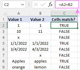
The simplest method to compare two cells in Excel is using the equals operator (=). This operator checks if the values in two cells are identical, returning TRUE if they are and FALSE otherwise.

=A1=B1

This formula directly compares the values in cell A1 and cell B1.

Example:

• If A1 contains “apple” and B1 contains “apple”, the formula returns TRUE.
• If A1 contains “apple” and B1 contains “orange”, the formula returns FALSE.

1.2. Understanding Case Sensitivity

The equals operator (=) performs a case-insensitive comparison. This means it treats uppercase and lowercase letters as the same. For example, “apple” and “Apple” would be considered equal.

Example:

• If A1 contains “Apple” and B1 contains “apple”, the formula =A1=B1 returns TRUE.

1.3. Using the IF Function for Conditional Outcomes

The IF function allows you to return different values based on whether the comparison is true or false. The basic syntax is:

=IF(logical_test, value_if_true, value_if_false)

• logical_test: The comparison you want to make (e.g., A1=B1).
• value_if_true: The value to return if the comparison is true.
• value_if_false: The value to return if the comparison is false.

Example:

=IF(A1=B1, "Match", "No Match")

This formula compares the values in A1 and B1. If they are equal, it returns “Match”; otherwise, it returns “No Match”.

1.4. Returning a Value from Another Cell Based on the Comparison

You can also use the IF function to return the value from another cell if the comparison is true.

Example:

=IF(A1=B1, C1, "")

This formula checks if A1 and B1 are equal. If they are, it returns the value in C1; otherwise, it returns an empty string (“”).

1.5. Case-Sensitive Comparison Using the EXACT Function

To perform a case-sensitive comparison, use the EXACT function. This function checks if two strings are exactly the same, including case.

=EXACT(A1, B1)

This formula returns TRUE if A1 and B1 are exactly the same (including case) and FALSE otherwise.

Example:

• If A1 contains “Apple” and B1 contains “apple”, the formula =EXACT(A1, B1) returns FALSE.
• If A1 contains “apple” and B1 contains “apple”, the formula =EXACT(A1, B1) returns TRUE.

You can combine the EXACT function with the IF function for conditional outcomes:

=IF(EXACT(A1, B1), "Match", "No Match")

This formula returns “Match” only if A1 and B1 are exactly the same (including case), and “No Match” otherwise.

2. Comparing One Cell to Multiple Cells: Techniques and Formulas

When you need to compare a single cell against a range of cells, Excel provides several techniques to accomplish this efficiently. These methods allow you to identify if the single cell’s value exists within the range, find matches, or perform more complex analyses.

2.1. Using the OR Function to Check for a Match in Multiple Cells

The OR function checks if at least one of the conditions is true. You can use it to compare a single cell against multiple cells, returning TRUE if there is a match.

=OR(A1=B1, A1=C1, A1=D1)

This formula checks if the value in A1 is equal to the value in B1, C1, or D1. If any of these comparisons are true, the formula returns TRUE; otherwise, it returns FALSE.

Example:

• If A1 contains “apple”, B1 contains “orange”, C1 contains “apple”, and D1 contains “banana”, the formula returns TRUE because A1 matches C1.
• If A1 contains “apple”, and B1, C1, and D1 contain “orange”, “banana”, and “grape” respectively, the formula returns FALSE.

For Excel 365 and later versions, you can simplify this using array formulas:

=OR(A1=B1:D1)

This formula performs the same comparison as the previous one but uses a more compact syntax. Note that in older versions of Excel (2019 and earlier), you may need to enter this as an array formula by pressing Ctrl + Shift + Enter.

2.2. Using the COUNTIF Function to Find Matches in a Range

The COUNTIF function counts the number of cells within a range that meet a given criterion. You can use it to check if a single cell’s value appears in a range of cells.

=COUNTIF(B1:D1, A1)>0

This formula counts the number of cells in the range B1:D1 that are equal to the value in A1. If the count is greater than 0, it means there is at least one match, and the formula returns TRUE; otherwise, it returns FALSE.

Example:

• If A1 contains “apple”, B1 contains “orange”, C1 contains “apple”, and D1 contains “banana”, the formula returns TRUE because “apple” appears once in the range B1:D1.
• If A1 contains “apple”, and B1, C1, and D1 contain “orange”, “banana”, and “grape” respectively, the formula returns FALSE.

2.3. Combining IF with OR or COUNTIF for Custom Outcomes

You can combine the IF function with either OR or COUNTIF to return custom values based on whether a match is found.

Using IF with OR:

=IF(OR(A1=B1, A1=C1, A1=D1), "Match Found", "No Match")

This formula checks if A1 matches any of the cells in B1, C1, or D1. If there is a match, it returns “Match Found”; otherwise, it returns “No Match”.

Using IF with COUNTIF:

=IF(COUNTIF(B1:D1, A1)>0, "Match Found", "No Match")

This formula does the same as the previous one but uses the COUNTIF function to check for a match.

2.4. Case-Sensitive Comparison with EXACT and Array Formulas

To perform a case-sensitive comparison when checking if a single cell matches any cell in a range, you can use the EXACT function in combination with an array formula.

=OR(EXACT(A1, B1:D1))

This formula checks if A1 is exactly the same as any of the cells in B1:D1, including case. In older versions of Excel (2019 and earlier), you need to enter this as an array formula by pressing Ctrl + Shift + Enter.

Example:

• If A1 contains “Apple”, B1 contains “apple”, C1 contains “Apple”, and D1 contains “banana”, the formula returns TRUE because A1 matches C1 exactly.
• If A1 contains “apple”, and B1, C1, and D1 contain “Apple”, “banana”, and “grape” respectively, the formula returns FALSE.

You can also combine this with the IF function for custom outcomes:

=IF(OR(EXACT(A1, B1:D1)), "Exact Match Found", "No Exact Match")

This formula returns “Exact Match Found” only if A1 is exactly the same as one of the cells in B1:D1, including case; otherwise, it returns “No Exact Match”.

2.5. Using MATCH Function to Find the Position of the Matching Cell

The MATCH function searches for a specified item in a range of cells, and then returns the relative position of that item in the range.

=MATCH(A1,B1:D1,0)

• A1: The value you want to search for.
• B1:D1: The range of cells you want to search in.
• 0: Specifies an exact match.

Example:

• If A1 contains “apple”, B1 contains “orange”, C1 contains “apple”, and D1 contains “banana”, the formula returns 2 because “apple” is found at the second position in the range B1:D1.
• If A1 contains “apple”, and B1, C1, and D1 contain “orange”, “banana”, and “grape” respectively, the formula returns #N/A, indicating that the value was not found.

You can combine this with ISNUMBER function to check if a match is found:

=IF(ISNUMBER(MATCH(A1,B1:D1,0)), "Match Found", "No Match")

This formula returns “Match Found” only if A1 is found in one of the cells in B1:D1; otherwise, it returns “No Match”.

3. Comparing Ranges and Arrays

In addition to comparing individual cells, Excel allows you to compare entire ranges or arrays. This can be useful for identifying differences, similarities, or patterns between datasets.

3.1. Comparing Two Ranges for Equality

To compare two ranges cell-by-cell and determine if they are identical, you can use the AND function in combination with an array formula.

=AND(A1:A3=B1:B3)

This formula compares each cell in the range A1:A3 with the corresponding cell in the range B1:B3. It returns TRUE only if all the corresponding cells are equal; otherwise, it returns FALSE. Note that you may need to enter this as an array formula by pressing Ctrl + Shift + Enter in older versions of Excel (2019 and earlier).

Example:

• If A1:A3 contains “apple”, “banana”, “orange” and B1:B3 contains “apple”, “banana”, “orange”, the formula returns TRUE.
• If A1:A3 contains “apple”, “banana”, “orange” and B1:B3 contains “apple”, “grape”, “orange”, the formula returns FALSE.

You can also combine this with the IF function for custom outcomes:

=IF(AND(A1:A3=B1:B3), "Ranges Match", "Ranges Differ")

This formula returns “Ranges Match” only if all corresponding cells in A1:A3 and B1:B3 are equal; otherwise, it returns “Ranges Differ”.

3.2. Identifying Differences Between Two Ranges

To identify the specific cells that differ between two ranges, you can use conditional formatting.

1. Select the range you want to compare (e.g., A1:A3).
2. Go to Home > Conditional Formatting > New Rule.
3. Select “Use a formula to determine which cells to format”.
4. Enter the following formula:

=A1<>B1

(Adjust the cell references as needed to match the top-left cell of your selected range and the corresponding cell in the other range.)

5. Click Format and choose the formatting you want to apply to the differing cells (e.g., a fill color).
6. Click OK twice.

This will highlight the cells in the selected range that do not match the corresponding cells in the comparison range.

3.3. Using Array Formulas for More Complex Comparisons

Array formulas can be used to perform more complex comparisons between ranges or arrays. For example, you can use them to count the number of cells that differ between two ranges.

=SUM(IF(A1:A3<>B1:B3, 1, 0))

This formula compares each cell in the range A1:A3 with the corresponding cell in the range B1:B3. If the cells are different, it returns 1; otherwise, it returns 0. The SUM function then adds up all the 1s, giving you the total number of differing cells. Remember to enter this as an array formula by pressing Ctrl + Shift + Enter in older versions of Excel (2019 and earlier).

Example:

• If A1:A3 contains “apple”, “banana”, “orange” and B1:B3 contains “apple”, “grape”, “orange”, the formula returns 1 because one cell differs.
• If A1:A3 contains “apple”, “banana”, “orange” and B1:B3 contains “apple”, “banana”, “orange”, the formula returns 0.

3.4. Transposing Data for Vertical Comparisons

Sometimes, your data might be arranged vertically instead of horizontally. In such cases, you can use the TRANSPOSE function to switch rows into columns or vice versa for easier comparison.

=TRANSPOSE(A1:A3)

This function converts the vertical range A1:A3 into a horizontal array that can be compared with another horizontal array using the methods described above.

4. Practical Examples and Use Cases

To illustrate the practical applications of comparing cells in Excel, let’s examine some real-world examples and use cases.

4.1. Data Validation: Ensuring Consistency

Data validation is a critical step in maintaining data integrity. By comparing cells and ranges, you can ensure that data is consistent across your spreadsheets.

Scenario:

You have two columns of product IDs, and you want to ensure that all the IDs in column A also exist in column B.

Solution:

1. In column C, enter the formula:

=IF(COUNTIF(B:B, A1)>0, "Valid", "Invalid")

2. Copy the formula down column C.

This formula checks if each product ID in column A exists in column B. If it does, it returns “Valid”; otherwise, it returns “Invalid”.

4.2. Inventory Management: Tracking Stock Levels

Comparing cells can help you manage your inventory by tracking stock levels and identifying discrepancies.

Scenario:

You have a list of products in column A, their current stock levels in column B, and their reorder points in column C. You want to identify which products need to be reordered.

Solution:

1. In column D, enter the formula:

=IF(B1<=C1, "Reorder", "")

2. Copy the formula down column D.

This formula checks if the current stock level (column B) is less than or equal to the reorder point (column C). If it is, it returns “Reorder”; otherwise, it returns an empty string.

4.3. Financial Analysis: Comparing Budgets to Actuals

Comparing cells is essential for financial analysis, allowing you to compare budgets to actual spending and identify variances.

Scenario:

You have a budget in column A and actual spending in column B. You want to calculate the variance and identify significant deviations.

Solution:

1. In column C, enter the formula:

=B1-A1

This calculates the variance (actual spending minus budget).

2. In column D, enter the formula:

=IF(ABS(C1)>0.1*A1, "Significant", "")

This checks if the absolute value of the variance is greater than 10% of the budget. If it is, it returns “Significant”; otherwise, it returns an empty string.

4.4. Identifying Duplicate Entries

Finding duplicate entries is a common task in data cleaning.

Scenario:

You have a list of email addresses in column A and want to identify any duplicates.

Solution:

1. In column B, enter the formula:

=IF(COUNTIF(A:A, A1)>1, "Duplicate", "")

2. Copy the formula down column B.

This formula counts how many times each email address appears in column A. If it appears more than once, it returns “Duplicate”; otherwise, it returns an empty string.

4.5. Comparing Data from Different Sources

Often, you need to compare data from different sources to identify discrepancies or ensure consistency.

Scenario:

You have customer data from two different databases in two separate Excel sheets. You want to compare the customer IDs to find any missing or mismatched entries.

Solution:

1. In the first sheet (e.g., “Database1”), add a column to check against the second sheet.
2. Enter the formula:

=IF(COUNTIF(Database2!A:A, A1)>0, "Match", "Missing in Database2")

(Assuming customer IDs are in column A of both sheets.)

3. Copy the formula down the column.

This formula checks if each customer ID in “Database1” exists in “Database2”. If it does, it returns “Match”; otherwise, it returns “Missing in Database2”.

5. Advanced Techniques for Cell Comparison

Beyond the basic formulas and functions, Excel offers more advanced techniques for comparing cells and ranges, allowing you to handle complex scenarios and perform sophisticated analyses.

5.1. Using the SUMPRODUCT Function for Multiple Criteria

The SUMPRODUCT function can be used to compare cells based on multiple criteria. This is useful when you need to check for matches that meet several conditions.

Scenario:

You have a table with products in column A, their sizes in column B, and their colors in column C. You want to find the number of products that match a specific size and color.

Solution:

=SUMPRODUCT((A1:A10="Product1")*(B1:B10="Large")*(C1:C10="Red"))

This formula counts the number of rows where the product in column A is “Product1”, the size in column B is “Large”, and the color in column C is “Red”. The * operator acts as an AND condition, requiring all three criteria to be met.

5.2. Using the INDEX and MATCH Functions for Dynamic Comparisons

The INDEX and MATCH functions can be combined to perform dynamic comparisons, allowing you to look up values based on variable criteria.

Scenario:

You have a table with product names in column A and their prices in column B. You want to look up the price of a specific product entered in cell D1.

Solution:

=INDEX(B1:B10, MATCH(D1, A1:A10, 0))

This formula uses the MATCH function to find the row number of the product entered in D1 within the range A1:A10. The INDEX function then uses that row number to return the corresponding price from the range B1:B10.

5.3. Working with Dates and Times

When comparing cells containing dates and times, it’s important to understand how Excel stores these values and use appropriate formulas.

Scenario:

You have a list of dates in column A and want to check if each date is within the last 7 days from today’s date.

Solution:

=IF(A1>=TODAY()-7, "Within Last 7 Days", "Older")

This formula compares each date in column A with today’s date minus 7 days. If the date is within the last 7 days, it returns “Within Last 7 Days”; otherwise, it returns “Older”.

5.4. Comparing Text Strings with Wildcards

Excel allows you to use wildcards in text comparisons to match patterns rather than exact values.

• ?: Matches any single character.
• *: Matches any sequence of characters.

Scenario:

You have a list of product names in column A and want to identify products that start with “A”.

Solution:

=IF(LEFT(A1, 1)="A", "Starts with A", "")

Alternatively, you can use COUNTIF with wildcard.

=IF(COUNTIF(A1, "A*")>0, "Starts with A", "")

This formula checks if the first character of the product name in column A is “A”. If it is, it returns “Starts with A”; otherwise, it returns an empty string.

5.5. Using Custom Functions (UDFs) for Complex Comparisons

For very complex comparisons that cannot be easily achieved with built-in functions, you can create custom functions using VBA (Visual Basic for Applications).

Scenario:

You need to compare two cells based on a highly specific algorithm that is not available in Excel’s built-in functions.

Solution:

1. Open the VBA editor (Alt + F11).
2. Insert a new module (Insert > Module).
3. Write your custom function:

Function CustomCompare(cell1 As Range, cell2 As Range) As Boolean
    ' Add your custom comparison logic here
    If cell1.Value = cell2.Value Then
        CustomCompare = True
    Else
        CustomCompare = False
    End If
End Function

4. Use the custom function in your worksheet:

=CustomCompare(A1, B1)

This allows you to perform comparisons based on your own specific criteria and algorithms.

6. Best Practices for Cell Comparison

To ensure accuracy and efficiency when comparing cells in Excel, follow these best practices:

6.1. Ensure Data Consistency

Before comparing cells, ensure that the data is consistent in terms of formatting, data types, and values. Inconsistent data can lead to inaccurate comparisons.

• Formatting: Ensure that cells have the same formatting (e.g., number format, date format).
• Data Types: Ensure that cells contain the same data types (e.g., numbers, text, dates).
• Values: Ensure that values are entered consistently (e.g., avoid leading or trailing spaces).

6.2. Use Absolute and Relative References Appropriately

When copying formulas, use absolute references ($) to keep certain cell references constant and relative references to adjust cell references based on their position.

• Absolute Reference: $A$1 (the cell reference does not change when the formula is copied).
• Relative Reference: A1 (the cell reference changes relative to the position of the formula when copied).
• Mixed Reference: $A1 or A$1 (either the column or row reference is fixed).

6.3. Test Your Formulas Thoroughly

Before relying on your formulas, test them thoroughly with different scenarios to ensure they produce the correct results.

• Edge Cases: Test your formulas with edge cases (e.g., empty cells, zero values, maximum values).
• Sample Data: Test your formulas with a representative sample of your data.
• Manual Calculation: Manually calculate the expected results for a few cases and compare them with the formula results.

6.4. Document Your Formulas

Add comments to your formulas to explain their purpose and logic. This makes it easier to understand and maintain your spreadsheets.

• Use the N function to add comments to formulas without affecting their results:

=A1+B1+N("This formula calculates the sum of A1 and B1")

6.5. Use Named Ranges

Using named ranges can make your formulas more readable and easier to understand.

1. Select the range you want to name.
2. Go to the Formulas tab > Define Name.
3. Enter a name for the range and click OK.

You can then use the named range in your formulas:

=SUM(MyRange)

6.6. Check for Errors

Excel provides several error-checking tools to help you identify and correct errors in your formulas.

• Error Checking: Go to the Formulas tab > Error Checking.
• Trace Precedents and Dependents: Use these tools to visualize the relationships between cells and formulas.
• Evaluate Formula: Use this tool to step through the calculation of a formula and identify any errors.

7. Conclusion: Making Informed Decisions with Data Comparison

Mastering the techniques for comparing cells in Excel is essential for anyone working with data. Whether you’re validating data, managing inventory, analyzing financials, or identifying duplicates, these skills will enable you to make informed decisions and improve your productivity. Remember to leverage the power of functions like IF, OR, COUNTIF, EXACT, and SUMPRODUCT, and follow best practices to ensure accuracy and efficiency.

At COMPARE.EDU.VN, we understand the importance of data-driven decision-making. That’s why we provide comprehensive resources and tools to help you master Excel and other data analysis techniques. Visit our website at COMPARE.EDU.VN to explore more articles, tutorials, and resources that can help you unlock the full potential of your data.

Need help comparing products, services, or even educational institutions? COMPARE.EDU.VN is your go-to resource for unbiased and detailed comparisons. Visit us at 333 Comparison Plaza, Choice City, CA 90210, United States, or reach out via WhatsApp at +1 (626) 555-9090.

Ready to take your Excel skills to the next level? Browse COMPARE.EDU.VN for in-depth comparisons and make smarter decisions today.

8. Frequently Asked Questions (FAQ)

Q1: How do I compare two cells for an exact match, including case sensitivity?

Use the EXACT function. For example, =IF(EXACT(A1, B1), "Match", "No Match").

Q2: How can I compare one cell to multiple cells and return “Match” if any of them match?

Use the OR function with multiple comparisons or the COUNTIF function. For example, =IF(OR(A1=B1, A1=C1, A1=D1), "Match", "No Match") or =IF(COUNTIF(B1:D1, A1)>0, "Match", "No Match").

Q3: How do I check if two ranges are equal cell by cell?

Use the AND function with an array formula. For example, =AND(A1:A3=B1:B3) (enter with Ctrl + Shift + Enter in older Excel versions).

Q4: How can I identify the differences between two ranges?

Use conditional formatting with a formula like =A1<>B1 to highlight differing cells.

Q5: How do I compare dates and times in Excel?

Ensure that cells are formatted as dates or times and use comparison operators like =, <, >. For example, =IF(A1>TODAY(), "Future Date", "Past or Present").

Q6: Can I use wildcards in cell comparisons?

Yes, use the COUNTIF function with wildcards. For example, =IF(COUNTIF(A1, "A*")>0, "Starts with A", "").

Q7: How do I create a case-sensitive comparison for multiple cells?

Use the EXACT function in combination with OR or array formulas. For example, =IF(OR(EXACT(A1, B1:D1)), "Exact Match", "No Match") (enter with Ctrl + Shift + Enter in older Excel versions).

Q8: What is the best way to compare data from two different Excel sheets?

Use the COUNTIF function referencing the other sheet. For example, =IF(COUNTIF(Sheet2!A:A, A1)>0, "Match", "Missing in Sheet2").

Q9: How can I use a custom function to compare cells based on my own criteria?

Create a custom function using VBA (Visual Basic for Applications) in the VBA editor (Alt + F11).

Q10: Where can I find more resources and tutorials on Excel comparisons?

Visit compare.edu.vn for comprehensive guides, articles, and tutorials on Excel and other data analysis techniques.