How To Compare Names In Two Excel Columns?

Comparing names in two Excel columns is a common task for data cleaning, reconciliation, and analysis. At COMPARE.EDU.VN, we provide a variety of methods to accomplish this, depending on your specific needs and data structure, from simple row-by-row comparisons to more complex matching and highlighting techniques. This comprehensive guide offers step-by-step instructions and formulas, ensuring you can efficiently identify matches, mismatches, and missing data points. Let’s explore techniques using conditional formatting, lookup formulas, and even handling partial matches in your data sets.

1. Comparing Two Columns for Exact Row Match

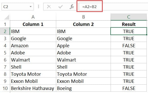
This method is suitable when you need to verify if the data in each row of two columns is identical. It’s a straightforward approach to identify matching or differing entries on a row-by-row basis.

1.1. Example: Compare Cells in the Same Row

Consider a dataset where you want to check if the name in column A is the same as the name in column B for each row. You can use a simple formula to achieve this.

Formula:

=A2=B2

This formula compares the values in cell A2 and B2. If they are the same, it returns “TRUE”; otherwise, it returns “FALSE.”

Comparing lists in Excel, with matches indicated as TRUE

1.2. Example: Compare Cells in the Same Row (Using IF Formula)

For a more descriptive result, you can use an IF formula to display “Match” or “Mismatch” instead of TRUE or FALSE.

Formula:

=IF(A2=B2,"Match","Mismatch")

This formula checks if A2 equals B2. If true, it returns “Match”; if false, it returns “Mismatch.”

Case-Sensitive Comparison:

If you need a case-sensitive comparison, use the EXACT function within the IF formula.

Formula:

=IF(EXACT(A2,B2),"Match","Mismatch")

With this formula, “IBM” and “ibm” would be considered different, and the formula would return “Mismatch.”

1.3. Example: Highlight Rows with Matching Data

Instead of displaying results in a separate column, you can highlight the rows with matching data using Conditional Formatting.

Steps:

1. Select the entire dataset.

2. Go to the “Home” tab.

   Click the Home Tab in the Excel ribbon

3. In the “Styles” group, click “Conditional Formatting.”

4. Click “New Rule.”

   Click on the New Rule option

5. Select “Use a formula to determine which cells to format.”

6. Enter the formula:

   =$A1=$B1

   Formula to compare columns in Conditional Formatting

7. Click “Format” and specify the desired formatting.

8. Click “OK.”

This will highlight all rows where the names in columns A and B match.

Comparing two columns and highlighting matching rows

2. Comparing Two Columns and Highlight Matches

This method focuses on identifying and highlighting data points that are present in both columns, regardless of their row position.

2.1. Example: Compare Two Columns and Highlight Matching Data

Often, datasets contain matches that are not in the same row. For example:

In this scenario, you want to highlight the matching company names (e.g., IBM, Adobe, Walmart).

Steps:

1. Select the entire dataset.

2. Go to the “Home” tab.

3. In the “Styles” group, click “Conditional Formatting.”

   Click on Conditional Formatting

4. Hover over “Highlight Cell Rules.”

5. Click “Duplicate Values.”

6. In the “Duplicate Values” dialog box, ensure “Duplicate” is selected.

   Duplicate in Conditional Formatting

7. Specify the formatting.

8. Click “OK.”

This will highlight all matching company names across both columns.

Highlighted matching data when comparing lists in Excel

Note: Conditional Formatting’s duplicate rule is not case-sensitive. “Apple” and “apple” will be considered the same and highlighted as duplicates.

2.2. Example: Compare Two Columns and Highlight Mismatched Data

To highlight names that are present in one list but not the other, use Conditional Formatting with the “Unique” option.

Steps:

1. Select the entire dataset.

2. Go to the “Home” tab.

3. In the “Styles” group, click “Conditional Formatting.”

4. Hover over “Highlight Cell Rules.”

5. Click “Duplicate Values.”

   Select Duplicate Values in Conditional Formatting

6. In the “Duplicate Values” dialog box, select “Unique.”

7. Specify the formatting.

   Specify the formatting to highlight differences in two columns

8. Click “OK.”

This will highlight all cells containing names that are not present in the other list, allowing you to quickly identify differences.

3. Comparing Two Columns and Find Missing Data Points

When you need to determine if a specific data point from one column is present in another, you can use lookup formulas like VLOOKUP or MATCH.

Suppose you have a dataset and you want to identify companies that are present in column A but not in column B.

Comparing two columns and highlighting matches – dataset

Using VLOOKUP:

Formula:

=ISERROR(VLOOKUP(A2,$B$2:$B$10,1,0))

This formula checks if the company name in A2 is present in column B. If the name is found, VLOOKUP returns the name; otherwise, it returns a #N/A error. The ISERROR function then returns TRUE if there is an error (i.e., the name is missing) and FALSE if not.

Using MATCH:

Formula:

=NOT(ISNUMBER(MATCH(A2,$B$2:$B$10,0)))

This formula uses the MATCH function to find the position of the company name in A2 within column B. If a match is found, MATCH returns the position; otherwise, it returns a #N/A error. The ISNUMBER function checks if the result is a number (i.e., a match was found), and NOT inverts the result, returning TRUE if there is no match and FALSE if there is a match.

To get a list of all missing names, filter the result column to show all cells with TRUE.

4. Comparing Two Columns and Pull the Matching Data

If you need to compare items in one column to another and retrieve corresponding data, lookup formulas are essential.

4.1. Example: Pull the Matching Data (Exact)

For instance, in the following list, you want to fetch the market valuation for each company in column D by looking up the company name in column A and retrieving the corresponding valuation from column B.

Comparing two lists in Excel and fetching matching data

Using VLOOKUP:

Formula:

=VLOOKUP(D2,$A$2:$B$14,2,0)

This formula searches for the value in D2 within the range A2:A14 and returns the corresponding value from the second column (market valuation) in the range A2:B14.

Using INDEX and MATCH:

Formula:

=INDEX($A$2:$B$14,MATCH(D2,$A$2:$A$14,0),2)

This formula first uses MATCH to find the row number where the value in D2 is located within the range A2:A14. Then, INDEX uses this row number to return the value from the second column (market valuation) in the range A2:B14.

4.2. Example: Pull the Matching Data (Partial)

When dealing with datasets where there are minor discrepancies in the names between two columns, standard lookup formulas may not work due to their need for exact matches. For example:

Pulling matching data – partial match

In such cases, you can use wildcard characters to perform a partial lookup.

Using VLOOKUP with Wildcards:

Formula:

=VLOOKUP("*"&D2&"*",$A$2:$B$14,2,0)

Using INDEX and MATCH with Wildcards:

Formula:

=INDEX($A$2:$B$14,MATCH("*"&D2&"*",$A$2:$A$14,0),2)

In these formulas, the asterisk (*) is a wildcard character that represents any number of characters. By flanking the lookup value with asterisks, the formula will consider any value in Column 1 that contains the lookup value in Column 2 as a match. For example, “*Exxon*” will match “ExxonMobil.”

5. Advanced Techniques for Comparing Names in Excel

Beyond the basic methods, advanced techniques can provide more nuanced and powerful comparisons.

5.1. Fuzzy Matching

Fuzzy matching is useful when you need to compare names that are similar but not identical due to typos, abbreviations, or variations in spelling. This technique uses algorithms to calculate the similarity between two strings and identify matches based on a similarity threshold.

Using the Fuzzy Lookup Add-In:

Microsoft offers a free add-in called “Fuzzy Lookup” that can be used for fuzzy matching in Excel.

Steps:

1. Download and install the Fuzzy Lookup Add-In from Microsoft.
2. Open Excel and go to the “Fuzzy Lookup” tab.
3. Select the two tables you want to compare.
4. Choose the columns to match (e.g., name columns).
5. Adjust the similarity threshold as needed.
6. Click “Go” to perform the fuzzy lookup.

The add-in will return a new table with the best matches and a similarity score for each match.

5.2. Using Array Formulas

Array formulas can perform complex calculations and comparisons across multiple cells. They are particularly useful for comparing lists and identifying matches based on multiple criteria.

Example: Finding Names in Column A That Are Not in Column B (Case-Sensitive):

Formula:

=IFERROR(INDEX($A$2:$A$10,MATCH(FALSE,ISNUMBER(MATCH($A$2:$A$10,$B$2:$B$10,0)),0)),"")

This is an array formula, so you must press Ctrl + Shift + Enter after entering it.

Explanation:

1. MATCH($A$2:$A$10,$B$2:$B$10,0): This part tries to find each name in column A within column B. It returns the position of the match if found, and #N/A if not found.
2. ISNUMBER(MATCH($A$2:$A$10,$B$2:$B$10,0)): This checks if the result of the MATCH function is a number (i.e., a match was found). It returns TRUE if a match is found and FALSE if not.
3. MATCH(FALSE,ISNUMBER(...),0): This looks for the first FALSE in the array of TRUE/FALSE values. It returns the position of the first FALSE, which corresponds to the first name in column A that is not found in column B.
4. INDEX($A$2:$A$10,MATCH(...),0): This returns the actual name from column A that is not found in column B.
5. IFERROR(...,""): If no name is found (i.e., all names in column A are in column B), the formula returns an empty string to avoid an error.

5.3. Using Power Query

Power Query (Get & Transform Data in Excel 2016 and later) is a powerful tool for data cleaning, transformation, and comparison. It can be used to compare names in two columns, merge data from different sources, and perform advanced filtering and grouping.

Steps:

1. Select the data in each column and convert it into a table (Insert > Table).
2. Go to Data > From Table/Range to open Power Query Editor.
3. In Power Query Editor, select the first table, then go to Merge Queries.
4. Choose the second table to merge with.
5. Select the column to match in both tables (e.g., name columns).
6. Choose the join kind (e.g., Left Anti to find names only in the first table).
7. Expand the merged column to bring in additional data or filter based on the merge result.
8. Close & Load the result into a new sheet.

6. Best Practices for Comparing Names in Excel

• Standardize Data: Ensure that the names in both columns are standardized before comparison. This includes removing extra spaces, converting to the same case (upper or lower), and removing punctuation.
• Use Helper Columns: Create helper columns to perform intermediate calculations or transformations. This can make complex formulas easier to understand and debug.
• Test Thoroughly: Always test your formulas and conditional formatting rules thoroughly to ensure they are working correctly. Use a variety of test cases, including matches, mismatches, and edge cases.
• Handle Errors: Use error-handling functions like IFERROR to gracefully handle errors and avoid displaying unsightly error messages in your worksheet.
• Document Your Work: Add comments to your formulas and conditional formatting rules to explain what they do. This will make it easier for you and others to understand and maintain your work.

7. Real-World Applications of Comparing Names in Excel

• Data Cleaning: Identifying and correcting inconsistencies in name fields across different datasets.
• Customer Relationship Management (CRM): Matching customer names between different CRM systems to consolidate customer data.
• Human Resources: Comparing employee names between payroll and HR systems to ensure data accuracy.
• Finance: Reconciling vendor names between invoices and vendor databases.
• Sales: Identifying duplicate leads or contacts in sales databases.

8. Troubleshooting Common Issues

• Formulas Not Working: Double-check your formulas for typos, incorrect cell references, and incorrect syntax. Use the “Evaluate Formula” tool to step through the formula and identify the source of the error.
• Conditional Formatting Not Applying: Ensure that your conditional formatting rules are correctly set up and that the formula is evaluating correctly. Check the order of your rules, as the first rule that evaluates to TRUE will be applied.
• Slow Performance: Complex formulas and conditional formatting rules can slow down Excel. To improve performance, try reducing the size of your datasets, using helper columns, and avoiding volatile functions.
• Inconsistent Results: Inconsistent results can be caused by data inconsistencies, such as extra spaces or different case. Standardize your data before performing comparisons.

9. Automating Name Comparison in Excel

Automating name comparison in Excel can save time and reduce errors, especially when dealing with large datasets.

9.1. Using Macros (VBA)

Macros can automate repetitive tasks in Excel, including comparing names in two columns.

Example: Macro to Highlight Matching Names:

Sub CompareNames()
    Dim rng1 As Range, rng2 As Range, cell As Range

    ' Set the ranges to compare
    Set rng1 = Range("A2:A10")
    Set rng2 = Range("B2:B10")

    ' Loop through each cell in the first range
    For Each cell In rng1
        ' Check if the value in the cell exists in the second range
        If Application.WorksheetFunction.CountIf(rng2, cell.Value) > 0 Then
            ' If it exists, highlight the cell
            cell.Interior.Color = RGB(255, 255, 0) ' Yellow
        End If
    Next cell
End Sub

Steps:

1. Press Alt + F11 to open the VBA editor.
2. Insert a new module (Insert > Module).
3. Paste the code into the module.
4. Modify the range references to match your data.
5. Run the macro by pressing F5 or clicking the “Run” button.

9.2. Using Power Automate

Power Automate (formerly Microsoft Flow) can automate tasks between Excel and other applications, such as SharePoint, OneDrive, and email.

Example: Flow to Compare Names and Send Email:

1. Create a new flow in Power Automate.
2. Use the “When a file is created or modified” trigger to start the flow when the Excel file is updated.
3. Use the “Get rows” action to retrieve the data from the Excel file.
4. Use the “Compose” action to create an array of names from each column.
5. Use the “Intersect” action to find the common names between the two arrays.
6. Use the “Send an email” action to send an email with the list of matching names.

10. Frequently Asked Questions (FAQs)

Q1: How can I compare two columns in Excel for exact matches?

You can use the formula =A2=B2 to compare the values in cells A2 and B2. This will return TRUE if the values are identical and FALSE if they are different.

Q2: How do I perform a case-sensitive comparison in Excel?

Use the EXACT function within an IF formula, like this: =IF(EXACT(A2,B2),"Match","Mismatch"). This will distinguish between “Apple” and “apple.”

Q3: Can I highlight matching names in two columns without using a formula in a separate column?

Yes, use Conditional Formatting. Select your data, go to “Home” > “Conditional Formatting” > “Highlight Cell Rules” > “Duplicate Values,” and choose your formatting.

Q4: How can I find names in one column that are missing from another?

Use the VLOOKUP formula: =ISERROR(VLOOKUP(A2,$B$2:$B$10,1,0)). This will return TRUE for names in column A that are not in column B.

Q5: How do I pull matching data from one column to another based on a name match?

Use the VLOOKUP or INDEX/MATCH formulas. For example: =VLOOKUP(D2,$A$2:$B$14,2,0) or =INDEX($A$2:$B$14,MATCH(D2,$A$2:$A$14,0),2).

Q6: What if the names in my columns are slightly different, like “JPMorgan” vs. “JPMorgan Chase”?

Use wildcard characters with VLOOKUP or INDEX/MATCH. For example: =VLOOKUP("*"&D2&"*",$A$2:$B$14,2,0).

Q7: How can I ignore case when highlighting duplicate names?

Conditional Formatting’s duplicate rule is not case-sensitive by default. Ensure your data is standardized to either all uppercase or lowercase before applying the rule.

Q8: Is there a way to automate the comparison of names in Excel?

Yes, you can use macros (VBA) or Power Automate to automate the comparison process.

Q9: How can I use Power Query to compare names in two columns?

In Power Query Editor, merge the two tables on the name columns. You can then expand the merged column to bring in additional data or filter based on the merge result.

Q10: What should I do if my formulas are not working correctly?

Double-check your formulas for typos, incorrect cell references, and incorrect syntax. Use the “Evaluate Formula” tool to step through the formula and identify the source of the error.

Conclusion

Comparing names in two Excel columns can be accomplished through various methods, each suited to different scenarios. Whether you need exact matches, partial matches, or more advanced fuzzy matching, Excel provides the tools and techniques to get the job done. By following the steps outlined in this guide, you can efficiently compare names, identify inconsistencies, and ensure data accuracy.

Ready to make data-driven decisions with confidence? Visit COMPARE.EDU.VN today to explore our comprehensive comparison tools and resources. Make informed choices and achieve your goals with COMPARE.EDU.VN!

Contact Us:

Address: 333 Comparison Plaza, Choice City, CA 90210, United States
Whatsapp: +1 (626) 555-9090
Website: compare.edu.vn