**How to Compare Names in Two Columns in Excel?**

Comparing names in two columns in Excel can be a complex task, but COMPARE.EDU.VN simplifies the process by providing various techniques and strategies to streamline your data analysis workflow. Excel offers multiple methods, from utilizing built-in functions and conditional formatting to employing advanced formulas, making it easier to compare columns and uncover hidden patterns within your data, and all these methods are available at compare.edu.vn. Simplify data comparison, identify discrepancies, and maintain accurate records with our comprehensive guide.

1. Why Is Comparing Two Columns in Excel Important?

Excel spreadsheets are vital for data storage, manipulation, and informed decision-making, presenting information in a user-friendly manner. Data analysts rely on Excel to gather information that drives marketing and sales strategies. The integrity of data within cells is crucial, as its absence can affect calculations and linked spreadsheets.

In this context, comparing two columns in Excel becomes essential for data analysts to verify data integrity. Manual comparison is often time-consuming, but Excel offers efficient alternatives, such as displaying results as TRUE/FALSE, Match/Not Match, or custom messages, facilitating data validation and analysis.

2. How Can You Compare Two Columns in Excel Effectively?

When dealing with data spread across two columns, tables, or spreadsheets, the ability to compare them becomes paramount to identify missing or common data. The approach to comparison varies based on the desired outcome, and Excel offers several methods to achieve this:

• Highlighting unique or duplicate values in each column using functions.
• Displaying unique or duplicate values using conditional formatting or formulas.
• Performing row-by-row comparison.
• Utilizing LOOKUP formulas.

Each method offers a unique way to analyze and compare data, allowing users to choose the most suitable approach for their specific needs.

3. How to Compare Two Columns in Excel Using the Equals Operator?

Comparing two columns in Excel using the equals operator allows for a row-by-row comparison, identifying matching data and presenting the result as either “Match” or “Not Match.” For instance, the formula =A2=B2 can be used to ascertain matching data, with the result being returned as True or False.

To implement this, enter the formula into cell C2 and drag it down to the end of the table. The formula will return TRUE if the values in the compared rows are identical and FALSE if they differ. This approach provides a straightforward method to pinpoint matching data across two columns.

4. How to Compare Two Columns in Excel Using the IF Condition?

In Excel, you can leverage the IF condition to compare two columns. The formula =IF(A2=B2,”Match”,” ”) will return “Match” for rows with matching values, leaving other rows blank.

For identifying and displaying mismatching values, the formula =IF(A2=B2,”Match”,”Not a Match ”) can be used, providing an additional result when the IF condition is false.

To compare two columns for differences, replace the equals sign with the non-equality sign (<>), resulting in the formula =IF(A2<>B2,”Match”,”Not a Match ”).

These formulas offer versatile ways to compare columns based on different criteria, providing clear indications of matches or mismatches.

5. How to Compare Two Columns in Excel Using the EXACT() Function?

The EXACT() function is essential when you need to perform a case-sensitive comparison between two columns in Excel. It compares two text strings and returns TRUE if they are identical, including case, and FALSE otherwise. The syntax is =EXACT(text1, text2), where both text1 and text2 are required arguments.

Consider an example where columns A and B contain the text string “Nova Scotia,” but with different capitalization. Applying the formula =IF(A2=B2, “Match”, “Mismatch”) would yield a “Match” result because it is case-insensitive.

However, using the formula =IF(EXACT(A2, B2), “Match”, “Mismatch”) makes the IF condition case-sensitive, accurately identifying the difference in capitalization.

The EXACT() function returns either true or false, which is then evaluated by the IF condition. This method ensures precise matching, taking into account the case of the text strings.

6. How to Compare Two Columns in Excel Using Conditional Formatting?

Conditional formatting offers a visual method to compare two columns in Excel. Begin by navigating to Home → Styles → Conditional Formatting → Highlight Cell Rules → Duplicate Values. This opens a dialog box where you can specify the formatting conditions.

You can choose to apply formatting to Duplicate or Unique values. Select the desired option and then choose a formatting style, such as filling with color, changing text color, or altering the cell border.

The Custom Format option allows you to select a specific color not listed in the drop-down menu. To highlight unique values, select Unique from the drop-down list.

If you wish to remove the applied formatting, go to Conditional Formatting → Clear Rules → Clear Rules from Selected Cells.

Conditional formatting is useful when you prefer not to have a third column displaying comparison results. It visually highlights duplicate (matching) and unique (different) data, making it easy to identify rows with the same data. This method is particularly suitable for smaller tables, while larger spreadsheets may require more complex approaches.

7. How to Compare Two Columns Using Lookup Functions?

The LOOKUP function in Excel searches for a value in a row or column and returns a corresponding value from another row or column. There are several lookup functions, including HLOOKUP, VLOOKUP, and XLOOKUP.

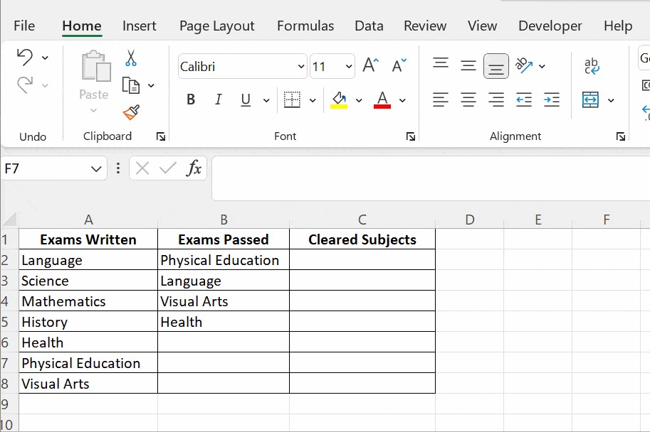
In the example below, we use VLOOKUP to compare two columns. Column A lists the exams taken by a student, and column B lists the subjects the student passed. To generate a result sheet, the formula =VLOOKUP(A2, $B$2:$B$5,1,0) is applied in cell C2.

Excel compare columns lookup function

Drag the formula down to apply it to all cells in column C. The result will display the cleared subjects, while those not cleared will show as #N/A. The components of the formula are as follows:

• VLOOKUP(A2,..,..,..) – Retrieves the value in cell A2.
• VLOOKUP(A2, $B$2:$B$5,..,..) – Compares with values in cells B2 to B5. The $ symbol creates an absolute reference, locking the cell range.
• VLOOKUP(A2, $B$2:$B$5,1,..) – Specifies the column index number, indicating the column position to compare from A2. In this case, it is 1 column away.
• VLOOKUP(A2, $B$2:$B$5,1,0) – The last argument is a logical value. Use 0 for an exact match and 1 for a close match sorted in ascending order.

8. How to Use the MATCH Function to Compare Two Columns?

The MATCH function in Excel is used to find the position of a specified value within a range of cells. It returns the relative position of the item in the array that matches a specified value in a specified order. The syntax for the MATCH function is:

=MATCH(lookup_value, lookup_array, [match_type])

• lookup_value: The value you want to find in the array.
• lookup_array: The range of cells being searched.
• [match_type]: Optional. Specifies how MATCH matches lookup_value with values in lookup_array. The possible values are -1, 0, or 1.

Example:

Suppose you have two columns of data: Column A contains a list of names, and Column B contains another list of names. You want to find out if the names in Column A appear in Column B and, if so, at what position.

	Column A	Column B
1	John	Alice
2	Alice	John
3	Bob	Bob
4	Charlie	David
5		Charlie

In Column C, you can use the MATCH function to check if each name in Column A exists in Column B:

	Column A	Column B	Column C
1	John	Alice	=MATCH(A1,B:B,0)
2	Alice	John	=MATCH(A2,B:B,0)
3	Bob	Bob	=MATCH(A3,B:B,0)
4	Charlie	David	=MATCH(A4,B:B,0)
5		Charlie

Here’s how the MATCH function works in this context:

• =MATCH(A1,B:B,0): This formula looks for the value in cell A1 (John) within all of Column B. The 0 specifies an exact match. If “John” is found in Column B, the formula returns the row number where it’s found. If not found, it returns #N/A.

• =MATCH(A2,B:B,0): This looks for the value in cell A2 (Alice) in Column B.

• =MATCH(A3,B:B,0): This looks for the value in cell A3 (Bob) in Column B.

• =MATCH(A4,B:B,0): This looks for the value in cell A4 (Charlie) in Column B.

The results in Column C would be:

	Column A	Column B	Column C
1	John	Alice	2
2	Alice	John	1
3	Bob	Bob	3
4	Charlie	David	5
5		Charlie

• 2: “John” is found in the second row of Column B.

• 1: “Alice” is found in the first row of Column B.

• 3: “Bob” is found in the third row of Column B.

• 5: “Charlie” is found in the fifth row of Column B.

Explanation:

1. Define Your Columns:

   • Column A has your first set of data (e.g., names, IDs).
   • Column B has your second set of data.

2. Write the Formula:

   • In an empty column (e.g., Column C), start writing the MATCH formula. For the first row, the formula might look like this:

   =MATCH(A1, B:B, 0)

   • A1 is the cell containing the first value you want to find in Column B.
   • B:B specifies that you want to search the entire Column B.
   • 0 requires an exact match.

3. Drag the Formula Down:

   • Drag the fill handle (the small square at the bottom-right of the cell) down to apply the formula to all rows in Column A.

Interpreting the Results:

• A Number: If the formula returns a number, that number indicates the row in Column B where the value from Column A is found. For example, if MATCH(A1, B:B, 0) returns 3, it means the value in A1 is found in the third row of Column B.
• #N/A: If the formula returns #N/A, it means the value from Column A is not found in Column B.

Additional Tips:

• Using with IF for Clarity:

  • To make the results more descriptive, you can wrap the MATCH function inside an IF function:

  =IF(ISNA(MATCH(A1, B:B, 0)), "Not Found", "Found")

  • ISNA checks if the result of MATCH is #N/A. If it is, the formula returns “Not Found”; otherwise, it returns “Found”.

• Highlighting Matches:

  • You can use conditional formatting to highlight the rows where matches are found. Create a new conditional formatting rule using a formula:

  =NOT(ISNA(MATCH(A1, B:B, 0)))

  • This formula checks if MATCH returns a value other than #N/A. If it does, the condition is true, and the cell is highlighted.

• Handling Large Datasets:

  • For very large datasets, consider using named ranges to improve performance. Instead of referencing entire columns (B:B), define a named range that covers only the relevant data.

Benefits:

• Verifies Data: Quickly check if data from one column exists in another.
• Identifies Differences: Easily spot missing or unmatched entries.
• Improves Accuracy: Helps ensure data consistency and reliability.
• Enhances Efficiency: Automates what would otherwise be a manual and time-consuming task.

By following these steps and understanding the nuances of the MATCH function, you can efficiently compare data in two columns in Excel, making data analysis and management more accurate and streamlined.

9. How to Compare Two Columns Using the COUNTIF Function?

The COUNTIF function in Excel is used to count the number of cells within a range that meet a given criterion. This can be particularly useful when comparing two columns to identify common or unique values. The syntax for the COUNTIF function is:

=COUNTIF(range, criteria)

• range: The range of cells you want to count.
• criteria: The condition that defines which cells will be counted.

Example:

Suppose you have two columns of data: Column A contains a list of names, and Column B contains another list of names. You want to find out how many names from Column A appear in Column B.

	Column A	Column B
1	John	Alice
2	Alice	John
3	Bob	Bob
4	Charlie	David
5	David	Charlie

In Column C, you can use the COUNTIF function to count how many times each name in Column A appears in Column B:

	Column A	Column B	Column C
1	John	Alice	=COUNTIF(B:B, A1)
2	Alice	John	=COUNTIF(B:B, A2)
3	Bob	Bob	=COUNTIF(B:B, A3)
4	Charlie	David	=COUNTIF(B:B, A4)
5	David	Charlie	=COUNTIF(B:B, A5)

Here’s how the COUNTIF function works in this context:

• =COUNTIF(B:B, A1): This formula counts how many times the value in cell A1 (John) appears within all of Column B.
• =COUNTIF(B:B, A2): This counts how many times the value in cell A2 (Alice) appears in Column B.
• =COUNTIF(B:B, A3): This counts how many times the value in cell A3 (Bob) appears in Column B.
• =COUNTIF(B:B, A4): This counts how many times the value in cell A4 (Charlie) appears in Column B.
• =COUNTIF(B:B, A5): This counts how many times the value in cell A5 (David) appears in Column B.

The results in Column C would be:

	Column A	Column B	Column C
1	John	Alice	1
2	Alice	John	1
3	Bob	Bob	1
4	Charlie	David	1
5	David	Charlie	1

Interpreting the Results:

• 1 or More: If the formula returns a number greater than 0, it means the value from Column A is found in Column B that many times.
• 0: If the formula returns 0, it means the value from Column A is not found in Column B.

Explanation:

1. Define Your Columns:

   • Column A has your first set of data (e.g., names, IDs).
   • Column B has your second set of data.

2. Write the Formula:

   • In an empty column (e.g., Column C), start writing the COUNTIF formula. For the first row, the formula might look like this:

   =COUNTIF(B:B, A1)

   • B:B specifies that you want to search the entire Column B.
   • A1 is the cell containing the first value you want to find in Column B.

3. Drag the Formula Down:

   • Drag the fill handle (the small square at the bottom-right of the cell) down to apply the formula to all rows in Column A.

Interpreting the Results:

• Greater Than 0: A number greater than 0 indicates that the value from Column A is found in Column B, and the number represents how many times it appears.
• 0: A result of 0 indicates that the value from Column A is not found in Column B.

Additional Tips:

• Using with IF for Clarity:

  • To make the results more descriptive, you can wrap the COUNTIF function inside an IF function:

  =IF(COUNTIF(B:B, A1)>0, "Found", "Not Found")

  • This formula checks if the count of the value in Column B is greater than 0. If it is, the formula returns “Found”; otherwise, it returns “Not Found”.

• Conditional Formatting:

  • You can use conditional formatting to highlight the rows where values from Column A are found in Column B. Create a new conditional formatting rule using a formula:

  =COUNTIF(B:B, A1)>0

  • Apply this rule to Column A. Excel will highlight the cells in Column A whose values are found in Column B.

• Handling Large Datasets:

  • For very large datasets, consider using named ranges to improve performance. Instead of referencing entire columns (B:B), define a named range that covers only the relevant data.

Benefits:

• Verifies Data: Quickly check if data from one column exists in another.
• Identifies Duplicates: Easily count how many times a value appears in the second column.
• Improves Accuracy: Helps ensure data consistency and reliability.
• Enhances Efficiency: Automates what would otherwise be a manual and time-consuming task.

By following these steps and understanding the nuances of the COUNTIF function, you can efficiently compare data in two columns in Excel, making data analysis and management more accurate and streamlined.

10. How to Compare Two Columns Using Array Formulas?

Array formulas in Excel are powerful tools that can perform complex calculations across multiple cells at once. When comparing two columns, array formulas can help identify matches, mismatches, or perform more advanced comparisons that standard formulas might not handle easily.

Understanding Array Formulas:

• What They Are: Array formulas operate on arrays (ranges of cells) rather than single values. They can perform calculations on each element in the array and return either a single result or an array of results.
• How to Enter: After typing the formula, you must press Ctrl + Shift + Enter to enter it as an array formula. Excel will automatically add curly braces {} around the formula to indicate that it is an array formula. Do not type the curly braces manually.

Example 1: Identifying Matching Rows

Suppose you have two columns of data and you want to identify which rows have matching entries.

	Column A	Column B
1	John	John
2	Alice	Alicia
3	Bob	Bob
4	Charlie	Charles
5	David	David

In Column C, you can use an array formula to check if each row has matching entries:

	Column A	Column B	Column C
1	John	John	=IF(A1:A5=B1:B5, "Match", "Mismatch")
2	Alice	Alicia	(Entered as an array formula using Ctrl+Shift+Enter)
3	Bob	Bob
4	Charlie	Charles
5	David	David

Steps:

1. Select the Output Range: Select the range of cells where you want the results to appear (e.g., C1:C5).

2. Enter the Formula: Type the following formula in the formula bar:

   =IF(A1:A5=B1:B5, "Match", "Mismatch")

3. Enter as Array Formula: Press Ctrl + Shift + Enter. Excel will add curly braces around the formula:

   {=IF(A1:A5=B1:B5, "Match", "Mismatch")}

The results in Column C would be:

	Column A	Column B	Column C
1	John	John	Match
2	Alice	Alicia	Mismatch
3	Bob	Bob	Match
4	Charlie	Charles	Mismatch
5	David	David	Match

Example 2: Finding Unique Values in Column A That Are Not in Column B

Suppose you want to find the values in Column A that do not appear in Column B.

	Column A	Column B
1	John	Alice
2	Alice	John
3	Bob	Bob
4	Charlie	David
5	David	Charlie

You can use an array formula with COUNTIF to achieve this. In Column C, enter the following formula as an array formula:

	Column A	Column B	Column C
1	John	Alice	=IF(COUNTIF(B:B, A1)=0, A1, "")
2	Alice	John	(Entered as an array formula using Ctrl+Shift+Enter)
3	Bob	Bob
4	Charlie	David
5	David	Charlie

Steps:

1. Select the Output Range: Select the range of cells where you want the results to appear (e.g., C1:C5).

2. Enter the Formula: Type the following formula in the formula bar:

   =IF(COUNTIF(B:B, A1)=0, A1, "")

3. Enter as Array Formula: Press Ctrl + Shift + Enter.

The results in Column C would be:

	Column A	Column B	Column C
1	John	Alice
2	Alice	John
3	Bob	Bob
4	Charlie	David
5	David	Charlie

Any cell in Column C that shows a name means that name from Column A is not found in Column B.

Key Considerations:

• Ctrl + Shift + Enter: Always remember to use Ctrl + Shift + Enter to enter the formula as an array formula.
• Performance: Array formulas can be resource-intensive, especially with large datasets. Use them judiciously.
• Understanding: Ensure you understand how the formula works to avoid errors and ensure correct results.

Benefits:

• Complex Comparisons: Handle comparisons that standard formulas can’t easily manage.
• Efficiency: Perform calculations across multiple cells simultaneously.
• Flexibility: Adapt to various data comparison needs.

By understanding and utilizing array formulas, you can significantly enhance your ability to compare data in two columns in Excel, making data analysis and management more powerful and efficient.

11. How to Compare Two Columns Using the INDEX-MATCH Function?

The INDEX and MATCH functions are often used together in Excel as a more flexible and powerful alternative to VLOOKUP. They can be particularly useful when comparing two columns and retrieving corresponding values based on matches.

Understanding the Functions:

• INDEX: Returns the value of a cell in a range (array) based on its row and column number.
  • Syntax: INDEX(array, row_num, [column_num])
• MATCH: Searches for a specified item in a range of cells and returns the relative position of that item in the range.
  • Syntax: MATCH(lookup_value, lookup_array, [match_type])

Example: Retrieving Corresponding Values

Suppose you have two columns of data in separate tables: Column A contains a list of IDs, and Column B contains corresponding names. Column D in another table also contains some IDs, and you want to retrieve the names from the first table that match the IDs in the second table.

	Column A (IDs)	Column B (Names)		Column D (IDs)	Column E (Retrieved Names)
1	101	John	1	102	=INDEX(B:B, MATCH(D1, A:A, 0))
2	102	Alice	2	104
3	103	Bob	3	101
4	104	Charlie	4	105
5	105	David	5

Steps:

1. Write the Formula:

   • In Column E, write the INDEX and MATCH formula to retrieve the corresponding names:

   =INDEX(B:B, MATCH(D1, A:A, 0))

   • MATCH(D1, A:A, 0): This part searches for the value in cell D1 (an ID) within Column A and returns its row number. The 0 specifies an exact match.
   • INDEX(B:B, ...): This part uses the row number returned by MATCH to retrieve the corresponding name from Column B.

2. Drag the Formula Down:

   • Drag the fill handle (the small square at the bottom-right of the cell) down to apply the formula to all rows in Column D.

Interpreting the Results:

• Name: If the formula returns a name, it means the ID from Column D was found in Column A, and the corresponding name from Column B is displayed.
• #N/A: If the formula returns #N/A, it means the ID from Column D was not found in Column A.

	Column A (IDs)	Column B (Names)		Column D (IDs)	Column E (Retrieved Names)
1	101	John	1	102	Alice
2	102	Alice	2	104	Charlie
3	103	Bob	3	101	John
4	104	Charlie	4	105	David
5	105	David	5

Explanation:

1. Define Your Tables:

   • Table 1 (Columns A and B) contains the master list of IDs and names.
   • Table 2 (Column D) contains a list of IDs for which you want to retrieve the names.

2. Write the Formula:

   • In the first row of your retrieval column (Column E), write the INDEX and MATCH formula:

   =INDEX(B:B, MATCH(D1, A:A, 0))

   • B:B is the column containing the names you want to retrieve.
   • D1 is the first ID you want to look up.
   • A:A is the column containing the IDs to search against.
   • 0 requires an exact match.

3. Drag the Formula Down:

   • Drag the fill handle down to apply the formula to all relevant rows.

Additional Tips:

• Handling Errors:

  • To handle cases where the ID is not found (resulting in #N/A), you can use the IFERROR function:

  =IFERROR(INDEX(B:B, MATCH(D1, A:A, 0)), "Not Found")

  • This will display “Not Found” instead of #N/A when there is no match.

• Named Ranges:

  • For better readability and performance, especially with large datasets, use named ranges. Define names for your ID column, name column, and lookup ID column.

  =INDEX(Names, MATCH(LookupID, IDs, 0))

Benefits:

• Flexibility: Works even when the lookup column is not the first column in the table.
• Efficiency: Fast and effective for retrieving corresponding values based on matches.
• Alternatives: More versatile than VLOOKUP, especially when column order might change.

By following these steps and understanding the nuances of the INDEX and MATCH functions, you can efficiently compare data in two columns and retrieve corresponding values, making data analysis and management more accurate and streamlined.

12. How To Compare Names In Two Columns With Slight Variations?

Comparing names in two columns when there are slight variations (e.g., typos, abbreviations, different formats) requires techniques that go beyond exact matching. Here’s a guide to help you with this task, combining several Excel functions and strategies.

1. Using the TRIM and CLEAN Functions

• Purpose: To remove extra spaces and non-printable characters.

• How to Use:

  =TRIM(CLEAN(A1))

  Apply this formula to both columns to standardize the data before comparison.

2. Using the LOWER or UPPER Functions

• Purpose: To ensure case consistency.

• How to Use:

  =LOWER(A1)

  or

  =UPPER(A1)

  Apply this to both columns to make the comparison case-insensitive.

3. Using the SUBSTITUTE Function

• Purpose: To replace specific characters or abbreviations.

• How to Use:

  =SUBSTITUTE(A1, "St.", "Street")

  Use this to replace common abbreviations or variations in names.

4. Using the SOUNDEX Function

• Purpose: To compare names based on how they sound rather than how they are spelled.

• How to Use:

  =SOUNDEX(A1)

  This function returns a four-character code representing how a word sounds. Compare the SOUNDEX codes of the names in both columns.

5. Using the FIND or SEARCH Functions

• Purpose: To find if one name contains a part of another name.

• How to Use:

  =IF(ISNUMBER(SEARCH(A1, B1)), "Match", "No Match")

  This checks if A1 is a substring of B1. SEARCH is case-insensitive and allows wildcards.

6. Using the LEFT and RIGHT Functions

• Purpose: To compare the first few characters of the names.

• How to Use:

  =IF(LEFT(A1, 3)=LEFT(B1, 3), "Match", "No Match")

  This compares the first 3 characters of the names.

7. Combining Functions for Robust Comparison

You can combine these functions for a more robust comparison. For example:

=IF(SOUNDEX(A1)=SOUNDEX(B1), "Likely Match",
    IF(ISNUMBER(SEARCH(A1, B1)), "Possible Match", "No Match"))

This formula first checks if the SOUNDEX codes match. If they do, it marks them as “Likely Match.” If not, it checks if A1 is a substring of B1