How To Compare Multiple Proportions: A Comprehensive Guide?

Comparing multiple proportions can be a challenge, but COMPARE.EDU.VN simplifies the process with comprehensive guides and resources, offering reliable methods for statistical analysis and decision-making. Explore our detailed articles to effortlessly navigate through proportion comparisons, ensuring well-informed choices.

1. Understanding Proportions and Their Importance

Proportions are a fundamental concept in statistics, representing the fraction of a population that possesses a specific characteristic. They are essential for understanding and comparing different groups or categories within a dataset.

1.1. What Is a Proportion?

A proportion is a ratio that compares a part to a whole. It is typically expressed as a decimal or percentage, indicating the fraction of a population that exhibits a particular trait or characteristic. For example, if 60 out of 200 students prefer online learning, the proportion of students who prefer online learning is 60/200 = 0.3 or 30%.

1.2. Why Compare Proportions?

Comparing proportions is crucial for various reasons:

Identifying Differences: It helps identify significant differences between groups or categories.
Informing Decisions: It supports data-driven decision-making in fields like healthcare, marketing, and social sciences.
Evaluating Interventions: It allows the evaluation of the effectiveness of different interventions or treatments.
Assessing Trends: It enables the assessment of changes and trends over time.

1.3. Real-World Applications of Proportion Comparison

Here are a few real-world applications:

Healthcare: Comparing the proportion of patients responding to different treatments.
Marketing: Assessing the success rate of different advertising campaigns.
Education: Comparing graduation rates between different educational programs.
Politics: Analyzing voter preferences across different demographics.
Manufacturing: Evaluating defect rates in different production processes.

2. Key Concepts in Comparing Proportions

Before diving into the methods for comparing multiple proportions, it’s essential to understand some key concepts that underpin these analyses.

2.1. Null and Alternative Hypotheses

In statistical hypothesis testing, the null hypothesis ((H_0)) is a statement of no effect or no difference, while the alternative hypothesis ((H_a)) is a statement that contradicts the null hypothesis.

Null Hypothesis ((H_0)): This hypothesis assumes that there is no significant difference between the proportions being compared. For example, (H_0: p_1 = p_2 = p_3), where (p_1, p_2, p_3) are the proportions of three different groups.
Alternative Hypothesis ((H_a)): This hypothesis states that there is a significant difference between the proportions. It can be one-tailed (e.g., (H_a: p_1 > p_2)) or two-tailed (e.g., (H_a: p_1 neq p_2)).

2.2. Significance Level ((alpha))

The significance level ((alpha)) is the probability of rejecting the null hypothesis when it is actually true (Type I error). Common values for (alpha) are 0.05 (5%) and 0.01 (1%). A smaller (alpha) reduces the risk of a false positive but increases the risk of a false negative (Type II error).

2.3. P-Value

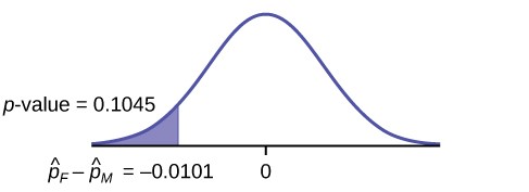
The p-value is the probability of observing a test statistic as extreme as, or more extreme than, the one computed from the sample data, assuming the null hypothesis is true. If the p-value is less than or equal to the significance level ((alpha)), the null hypothesis is rejected.

2.4. Test Statistic

A test statistic is a standardized value calculated from sample data during a hypothesis test. It is used to determine whether to reject the null hypothesis. The choice of test statistic depends on the specific test being performed.

2.5. Confidence Intervals

A confidence interval provides a range of values within which the true population proportion is likely to fall. It is calculated using the sample proportion and a margin of error, which is based on the desired level of confidence (e.g., 95% confidence interval).

3. Methods for Comparing Multiple Proportions

Several statistical methods can be used to compare multiple proportions, each with its own assumptions and applications. Here are some of the most common methods.

3.1. Chi-Square Test

The Chi-Square test is a versatile method used to determine if there is a significant association between two categorical variables. It compares the observed frequencies with the expected frequencies under the assumption of no association.

3.1.1. When to Use the Chi-Square Test

The Chi-Square test is appropriate when:

You have categorical data.
You want to determine if there is a significant association between two or more groups.
The sample sizes are sufficiently large (usually, each cell in the contingency table should have an expected count of at least 5).

3.1.2. How to Perform a Chi-Square Test

State the Hypotheses:
- Null Hypothesis ((H_0)): There is no association between the categorical variables.
- Alternative Hypothesis ((H_a)): There is an association between the categorical variables.
Create a Contingency Table:
- Organize the data into a table that shows the observed frequencies for each category.
Calculate Expected Frequencies:
- For each cell in the contingency table, calculate the expected frequency using the formula:
[
E_{ij} = frac{(text{Row Total}) times (text{Column Total})}{text{Grand Total}}
]
Calculate the Chi-Square Statistic:
- Compute the Chi-Square statistic using the formula:
[
chi^2 = sum frac{(O{ij} – E{ij})^2}{E_{ij}}
]

where (O{ij}) is the observed frequency and (E{ij}) is the expected frequency for each cell.
Determine the Degrees of Freedom:
- Calculate the degrees of freedom using the formula:
[
df = (r – 1) times (c – 1)
]

where (r) is the number of rows and (c) is the number of columns in the contingency table.
Find the P-Value:
- Use a Chi-Square distribution table or statistical software to find the p-value associated with the calculated Chi-Square statistic and degrees of freedom.
Make a Decision:
- If the p-value is less than or equal to the significance level ((alpha)), reject the null hypothesis. Otherwise, fail to reject the null hypothesis.

3.1.3. Example of Chi-Square Test

Suppose a marketing team wants to know if there is an association between the type of advertisement (online, print, TV) and the customer response (purchase, no purchase). The data is organized as follows:

	Purchase	No Purchase	Total
Online	80	120	200
Print	40	60	100
TV	60	40	100
Total	180	220	400

State the Hypotheses:
- (H_0): There is no association between the type of advertisement and customer response.
- (H_a): There is an association between the type of advertisement and customer response.
Calculate Expected Frequencies:
- For the Online/Purchase cell: (E_{11} = frac{200 times 180}{400} = 90)
- For the Online/No Purchase cell: (E_{12} = frac{200 times 220}{400} = 110)
- For the Print/Purchase cell: (E_{21} = frac{100 times 180}{400} = 45)
- For the Print/No Purchase cell: (E_{22} = frac{100 times 220}{400} = 55)
- For the TV/Purchase cell: (E_{31} = frac{100 times 180}{400} = 45)
- For the TV/No Purchase cell: (E_{32} = frac{100 times 220}{400} = 55)
Calculate the Chi-Square Statistic:

[
begin{aligned}
chi^2 &= frac{(80 – 90)^2}{90} + frac{(120 – 110)^2}{110} + frac{(40 – 45)^2}{45}
&+ frac{(60 – 55)^2}{55} + frac{(60 – 45)^2}{45} + frac{(40 – 55)^2}{55}
&= 1.11 + 0.91 + 0.56 + 0.45 + 5.00 + 4.09
&= 12.12
end{aligned}
]
Determine the Degrees of Freedom:
- (df = (3 – 1) times (2 – 1) = 2 times 1 = 2)
Find the P-Value:
- Using a Chi-Square distribution table or statistical software, the p-value for (chi^2 = 12.12) with (df = 2) is approximately 0.0023.
Make a Decision:
- Since the p-value (0.0023) is less than the significance level ((alpha = 0.05)), we reject the null hypothesis.
Conclusion:
- There is a significant association between the type of advertisement and customer response.

3.2. ANOVA for Proportions

ANOVA (Analysis of Variance) is typically used for comparing means, but it can be adapted for proportions when the proportions are transformed using the arcsine transformation.

3.2.1. When to Use ANOVA for Proportions

ANOVA for proportions is appropriate when:

You have more than two groups to compare.
The proportions are independent.
The sample sizes are sufficiently large.
The data are approximately normally distributed after arcsine transformation.

3.2.2. How to Perform ANOVA for Proportions

State the Hypotheses:
- Null Hypothesis ((H_0)): The proportions are equal across all groups.
- Alternative Hypothesis ((H_a)): At least one proportion is different from the others.
Transform the Proportions:
- Apply the arcsine transformation to each proportion:
[
p’ = arcsin(sqrt{p})
]

where (p) is the original proportion and (p’) is the transformed proportion.
Perform ANOVA on the Transformed Proportions:
- Calculate the F-statistic and p-value using standard ANOVA procedures.
Make a Decision:
- If the p-value is less than or equal to the significance level ((alpha)), reject the null hypothesis. Otherwise, fail to reject the null hypothesis.

3.2.3. Example of ANOVA for Proportions

Suppose a researcher wants to compare the success rates of three different teaching methods (A, B, C). The data is as follows:

	Success	Total	Proportion
Method A	75	150	0.50
Method B	90	150	0.60
Method C	60	150	0.40

State the Hypotheses:
- (H_0): The success rates are equal across all three methods.
- (H_a): At least one success rate is different from the others.
Transform the Proportions:
- For Method A: (p’_A = arcsin(sqrt{0.50}) approx 0.785)
- For Method B: (p’_B = arcsin(sqrt{0.60}) approx 0.886)
- For Method C: (p’_C = arcsin(sqrt{0.40}) approx 0.684)
Perform ANOVA on the Transformed Proportions:
- Using statistical software, perform ANOVA on the transformed proportions. Assume the ANOVA results in an F-statistic of 4.5 and a p-value of 0.02.
Make a Decision:
- Since the p-value (0.02) is less than the significance level ((alpha = 0.05)), we reject the null hypothesis.
Conclusion:
- There is a significant difference in the success rates among the three teaching methods.

3.3. Multiple Proportion Z-Test

The Multiple Proportion Z-Test extends the two-proportion Z-test to compare more than two proportions simultaneously. It is used to determine if there are significant differences among the proportions of several independent groups.

3.3.1. When to Use the Multiple Proportion Z-Test

The Multiple Proportion Z-Test is appropriate when:

You have more than two independent groups to compare.
The sample sizes are sufficiently large (typically, (n times p geq 5) and (n times (1-p) geq 5) for each group).
The data are categorical and can be represented as proportions.

3.3.2. How to Perform a Multiple Proportion Z-Test

State the Hypotheses:
- Null Hypothesis ((H_0)): All population proportions are equal ((p_1 = p_2 = dots = p_k)).
- Alternative Hypothesis ((H_a)): At least one population proportion is different from the others.
Calculate the Pooled Proportion:
- Combine the data from all groups to estimate the overall proportion:
[
bar{p} = frac{sum_{i=1}^{k} xi}{sum{i=1}^{k} n_i}
]

where (x_i) is the number of successes in group (i), and (n_i) is the sample size of group (i).
Calculate the Test Statistic:
- Compute the Z-statistic for each group:
[
Z_i = frac{p_i – bar{p}}{sqrt{bar{p}(1-bar{p})/n_i}}
]

where (p_i = frac{x_i}{n_i}) is the sample proportion for group (i).
Calculate the Chi-Square Statistic:
- Square each Z-statistic and sum them up to get the Chi-Square statistic:
[
chi^2 = sum_{i=1}^{k} Z_i^2
]
Determine the Degrees of Freedom:
- The degrees of freedom for this test are (df = k – 1), where (k) is the number of groups.
Find the P-Value:
- Use a Chi-Square distribution table or statistical software to find the p-value associated with the calculated Chi-Square statistic and degrees of freedom.
Make a Decision:
- If the p-value is less than or equal to the significance level ((alpha)), reject the null hypothesis. Otherwise, fail to reject the null hypothesis.

3.3.3. Example of Multiple Proportion Z-Test

Suppose a hospital wants to compare the infection rates across four different wards (A, B, C, D). The data is as follows:

	Infected	Total Patients	Proportion
Ward A	15	200	0.075
Ward B	20	250	0.080
Ward C	10	150	0.067
Ward D	25	300	0.083

State the Hypotheses:
- (H_0): The infection rates are equal across all four wards.
- (H_a): At least one infection rate is different from the others.
Calculate the Pooled Proportion:

[
bar{p} = frac{15 + 20 + 10 + 25}{200 + 250 + 150 + 300} = frac{70}{900} approx 0.078
]
Calculate the Test Statistic:
- For Ward A: (Z_A = frac{0.075 – 0.078}{sqrt{0.078(1-0.078)/200}} approx -0.166)
- For Ward B: (Z_B = frac{0.080 – 0.078}{sqrt{0.078(1-0.078)/250}} approx 0.118)
- For Ward C: (Z_C = frac{0.067 – 0.078}{sqrt{0.078(1-0.078)/150}} approx -0.517)
- For Ward D: (Z_D = frac{0.083 – 0.078}{sqrt{0.078(1-0.078)/300}} approx 0.326)
Calculate the Chi-Square Statistic:

[
chi^2 = (-0.166)^2 + (0.118)^2 + (-0.517)^2 + (0.326)^2 approx 0.439
]
Determine the Degrees of Freedom:
- (df = 4 – 1 = 3)
Find the P-Value:
- Using a Chi-Square distribution table or statistical software, the p-value for (chi^2 = 0.439) with (df = 3) is approximately 0.931.
Make a Decision:
- Since the p-value (0.931) is greater than the significance level ((alpha = 0.05)), we fail to reject the null hypothesis.
Conclusion:
- There is no significant difference in the infection rates among the four wards.

3.4. Cochran’s Q Test

Cochran’s Q test is a non-parametric test used to determine if there are significant differences among three or more related proportions. It is particularly useful when dealing with repeated measures or matched data.

3.4.1. When to Use Cochran’s Q Test

Cochran’s Q test is appropriate when:

You have three or more related groups (e.g., repeated measures on the same subjects).
The data are binary (success/failure) and can be represented as proportions.
The sample sizes are the same for each group.

3.4.2. How to Perform Cochran’s Q Test

State the Hypotheses:
- Null Hypothesis ((H_0)): The proportions are equal across all related groups.
- Alternative Hypothesis ((H_a)): At least one proportion is different from the others.
Create a Data Table:
- Organize the data into a table where each row represents a subject, and each column represents a related group.
Calculate the Test Statistic:
- Compute Cochran’s Q statistic using the formula:
[
Q = frac{(k – 1)[k sum_{j=1}^{k} Cj^2 – (sum{j=1}^{k} Cj)^2]}{k sum{i=1}^{n} Ri – sum{i=1}^{n} R_i^2}
]

where:
- (k) is the number of related groups.
- (C_j) is the column total for group (j).
- (R_i) is the row total for subject (i).
- (n) is the number of subjects.
Determine the Degrees of Freedom:
- The degrees of freedom for this test are (df = k – 1).
Find the P-Value:
- Use a Chi-Square distribution table or statistical software to find the p-value associated with the calculated Q statistic and degrees of freedom.
Make a Decision:
- If the p-value is less than or equal to the significance level ((alpha)), reject the null hypothesis. Otherwise, fail to reject the null hypothesis.

3.4.3. Example of Cochran’s Q Test

Suppose a researcher wants to compare the effectiveness of three different treatments (A, B, C) on the same group of patients. Each patient receives all three treatments in a random order, and the outcome is binary (success/failure). The data is as follows:

Patient	Treatment A	Treatment B	Treatment C	Row Total ((R_i))
1	1	0	1	2
2	0	0	1	1
3	1	1	1	3
4	0	1	0	1
5	1	0	0	1
Column Total ((C_j))	3	2	3

State the Hypotheses:
- (H_0): The treatments are equally effective.
- (H_a): At least one treatment is different from the others.
Calculate the Test Statistic:
- (k = 3) (number of treatments)
- (n = 5) (number of patients)
- (sum_{j=1}^{k} C_j^2 = 3^2 + 2^2 + 3^2 = 9 + 4 + 9 = 22)
- ((sum_{j=1}^{k} C_j)^2 = (3 + 2 + 3)^2 = 8^2 = 64)
- (sum_{i=1}^{n} R_i = 2 + 1 + 3 + 1 + 1 = 8)
- (sum_{i=1}^{n} R_i^2 = 2^2 + 1^2 + 3^2 + 1^2 + 1^2 = 4 + 1 + 9 + 1 + 1 = 16)
[
Q = frac{(3 – 1)[3(22) – (64)]}{3(8) – 16} = frac{2[66 – 64]}{24 – 16} = frac{2(2)}{8} = frac{4}{8} = 0.5
]
Determine the Degrees of Freedom:
- (df = 3 – 1 = 2)
Find the P-Value:
- Using a Chi-Square distribution table or statistical software, the p-value for (Q = 0.5) with (df = 2) is approximately 0.779.
Make a Decision:
- Since the p-value (0.779) is greater than the significance level ((alpha = 0.05)), we fail to reject the null hypothesis.
Conclusion:
- There is no significant difference in the effectiveness of the three treatments.

4. Practical Guide to Implementing Proportion Comparisons

To effectively compare multiple proportions, follow these practical steps:

4.1. Data Collection and Preparation

Collect Relevant Data: Ensure you have accurate and complete data for each group or category you want to compare.
Clean the Data: Remove any inconsistencies, errors, or missing values that could affect the results.
Organize the Data: Structure the data in a format suitable for statistical analysis, such as a contingency table or a dataset with proportions.

4.2. Choosing the Right Statistical Test

Consider the Number of Groups: If you are comparing two proportions, use a two-proportion Z-test. For more than two proportions, consider the Chi-Square test, ANOVA for proportions, or the Multiple Proportion Z-Test.
Assess Independence: If the groups are independent, use tests like Chi-Square or ANOVA. If the groups are related, use Cochran’s Q test.
Check Assumptions: Ensure that the assumptions of the chosen test are met, such as sufficient sample sizes and normality (if required).

4.3. Performing the Analysis

Use Statistical Software: Utilize tools like R, Python, SPSS, or SAS to perform the statistical analysis. These tools offer built-in functions for various proportion comparison tests.
Follow Step-by-Step Procedures: Adhere to the specific steps for each test, as outlined in the methods section.
Interpret the Results: Carefully interpret the p-values, test statistics, and confidence intervals to draw meaningful conclusions.

4.4. Interpreting Results and Drawing Conclusions

Evaluate Statistical Significance: Determine if the p-value is less than or equal to the significance level ((alpha)). If so, the results are statistically significant, and you can reject the null hypothesis.
Consider Practical Significance: Even if the results are statistically significant, assess whether the differences are practically meaningful in the real world.
Communicate Findings: Clearly communicate your findings using appropriate visualizations, tables, and narratives.

5. Advanced Considerations

For more complex scenarios, consider these advanced techniques:

5.1. Post-Hoc Tests

When ANOVA or Chi-Square tests indicate significant differences, post-hoc tests can be used to determine which specific groups differ from each other. Common post-hoc tests include:

Bonferroni Correction: Adjusts the significance level to account for multiple comparisons.
Tukey’s HSD (Honestly Significant Difference): Compares all possible pairs of means while controlling for the familywise error rate.
Dunn’s Test: A non-parametric post-hoc test for multiple comparisons.

5.2. Adjusting for Confounding Variables

Confounding variables can influence the relationship between proportions. Techniques to adjust for confounders include:

Stratified Analysis: Analyzing proportions within subgroups defined by the confounding variable.
Regression Analysis: Using regression models to control for the effects of confounding variables.

5.3. Bayesian Methods

Bayesian methods offer an alternative approach to proportion comparison, allowing for the incorporation of prior knowledge and the estimation of posterior probabilities. Bayesian hypothesis testing can provide more nuanced insights than traditional frequentist methods.

6. Common Pitfalls and How to Avoid Them

Comparing proportions can be tricky, and it’s easy to make mistakes. Here are some common pitfalls and how to avoid them:

6.1. Small Sample Sizes

Pitfall: Using tests designed for large samples on small datasets.
Solution: Ensure that you have sufficient sample sizes for each group. If sample sizes are small, consider using exact tests or Bayesian methods.

6.2. Violating Independence

Pitfall: Applying tests that assume independence to related data.
Solution: Use appropriate tests for related data, such as Cochran’s Q test.

6.3. Ignoring Assumptions

Pitfall: Failing to check the assumptions of the statistical tests.
Solution: Verify that the assumptions of the chosen test are met, such as normality (if required) and homogeneity of variances.

6.4. Overinterpreting Results

Pitfall: Drawing strong conclusions from statistically significant but practically insignificant results.
Solution: Consider both statistical and practical significance when interpreting results.

7. Case Studies: Real-World Examples

7.1. Marketing Campaign Analysis

A marketing team launches three different advertising campaigns (A, B, C) and wants to compare their effectiveness in generating leads. The data is as follows:

	Leads Generated	Total Impressions	Proportion
Campaign A	150	1000	0.15
Campaign B	180	1200	0.15
Campaign C	120	800	0.15

Using a Chi-Square test or Multiple Proportion Z-Test, the team can determine if there are significant differences in the lead generation rates among the three campaigns. Post-hoc tests can then be used to identify which specific campaigns differ from each other.

7.2. Healthcare Treatment Evaluation

A hospital is evaluating the success rates of three different treatments for a particular disease. The data is as follows:

	Success	Total Patients	Proportion
Treatment A	80	200	0.40
Treatment B	90	200	0.45
Treatment C	70	200	0.35

ANOVA for proportions can be used to compare the success rates across the three treatments. If significant differences are found, post-hoc tests can help identify which treatments are more effective than others.

7.3. Educational Program Assessment

A school district is assessing the graduation rates of three different educational programs. The data is as follows:

	Graduates	Total Students	Proportion
Program A	120	150	0.80
Program B	130	160	0.81
Program C	110	140	0.79

A Multiple Proportion Z-Test can be used to determine if there are significant differences in the graduation rates among the three programs. This information can help the school district make informed decisions about resource allocation and program improvements.

8. Frequently Asked Questions (FAQ)

Q1: What is a proportion, and why is it important to compare proportions?

A proportion is a ratio that compares a part to a whole. Comparing proportions is essential for identifying differences between groups, informing decisions, evaluating interventions, and assessing trends over time.

Q2: When should I use the Chi-Square test for comparing proportions?

Use the Chi-Square test when you have categorical data, want to determine if there is a significant association between two or more groups, and the sample sizes are sufficiently large.

Q3: What is ANOVA for proportions, and when is it appropriate to use?

ANOVA for proportions is an adaptation of ANOVA used to compare more than two proportions. It is appropriate when you have more than two independent groups, the sample sizes are sufficiently large, and the data are approximately normally distributed after arcsine transformation.

Q4: What is the Multiple Proportion Z-Test, and how does it work?

The Multiple Proportion Z-Test extends the two-proportion Z-test to compare more than two proportions simultaneously. It calculates a pooled proportion, computes Z-statistics for each group, and uses a Chi-Square statistic to determine if there are significant differences among the proportions.

Q5: When should I use Cochran’s Q test for comparing proportions?

Use Cochran’s Q test when you have three or more related groups (e.g., repeated measures), the data are binary (success/failure), and the sample sizes are the same for each group.

Q6: How do I choose the right statistical test for comparing proportions?

Consider the number of groups, assess independence, and check assumptions. Use the two-proportion Z-test for two groups, Chi-Square or ANOVA for multiple independent groups, and Cochran’s Q test for related groups.

Q7: What are post-hoc tests, and when should I use them?

Post-hoc tests are used after ANOVA or Chi-Square tests indicate significant differences. They determine which specific groups differ from each other, using methods like Bonferroni correction or Tukey’s HSD.

Q8: How can I adjust for confounding variables when comparing proportions?

Adjust for confounding variables using techniques like stratified analysis, analyzing proportions within subgroups, or regression analysis to control for the effects of confounders.

Q9: What are some common pitfalls to avoid when comparing proportions?

Common pitfalls include small sample sizes, violating independence, ignoring assumptions, and overinterpreting results. Ensure you have sufficient sample sizes, use appropriate tests for related data, verify assumptions, and consider both statistical and practical significance.

Q10: How can COMPARE.EDU.VN help me with comparing multiple proportions?

COMPARE.EDU.VN provides comprehensive guides, reliable methods, and resources for statistical analysis and decision-making. Our detailed articles help you navigate through proportion comparisons, ensuring well-informed choices.

9. Conclusion: Making Informed Decisions with Proportion Comparisons

Comparing multiple proportions is a powerful tool for understanding differences, evaluating interventions, and making informed decisions. By understanding the key concepts, choosing the right statistical methods, and avoiding common pitfalls, you can effectively use proportion comparisons to gain valuable insights from your data. Visit COMPARE.EDU.VN for more in-depth resources and tools to assist you in your comparative analyses.

Contingency table showing observed frequencies for each category

Are you struggling to compare different options and make the right choice? At compare.edu.vn, we understand the challenges you face. That’s why we provide detailed and objective comparisons across various products, services, and ideas. Our goal is to equip you with the information you need to make confident and informed decisions.

Whether you’re a student comparing educational resources, a