Comparing multiple cells in Excel is a common task for data analysis, financial modeling, and decision-making. At COMPARE.EDU.VN, we understand the need for simple and effective methods. This guide explores various techniques to compare multiple cells in Excel, providing you with the tools to make informed decisions.
1. Understanding the Need to Compare Multiple Cells in Excel
Excel is a powerful tool, but comparing data across multiple cells can be challenging. Whether you’re verifying data integrity, identifying discrepancies, or simply looking for patterns, knowing how to effectively compare cells is crucial. This comprehensive guide from COMPARE.EDU.VN will help you master these techniques, empowering you to make data-driven decisions.
2. Simple “If Two Cells Equal, Return TRUE” Formula
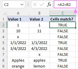
The most straightforward way to compare two cells is using a simple equality formula. This method returns TRUE if the cells match and FALSE if they don’t.
2.1. Basic Syntax
The basic formula is:
=cell A = cell B
For instance, if you want to compare cells A2 and B2, the formula would be:
=A2=B2
This formula checks if the value in cell A2 is equal to the value in cell B2.
2.2. Important Notes
- This formula returns a Boolean value: TRUE or FALSE.
- The comparison is case-insensitive, meaning it treats uppercase and lowercase letters as the same.
- To return only TRUE values, integrate it into an IF statement, as shown in the next section.
3. Returning a Specific Value if Cells Match
Instead of just TRUE or FALSE, you might want to return a specific value when cells match. This can be achieved using the IF function.
3.1. The IF Statement Structure
The general structure of the IF statement is:
=IF(cell A = cell B, value_if_true, value_if_false)
Here, value_if_true is the value returned if the cells match, and value_if_false is returned if they don’t.
3.2. Examples
- To return “yes” if A2 and B2 match, and “no” if they don’t:
=IF(A2=B2, "yes", "no")
- To return “yes” if they match, and leave the cell blank if they don’t:
=IF(A2=B2, "yes", "")
- To return the logical value TRUE if they match:
=IF(A2=B2, TRUE, "")
Note: Do not enclose TRUE in double quotes if you want to return the logical value.
4. Returning a Value from Another Cell If Cells Match
A more advanced scenario involves comparing two cells and, if they match, returning a value from a third cell.
4.1. Formula Structure
The formula structure for this is:
=IF(cell A = cell B, cell C, "")
Here, if cell A and cell B match, the value from cell C is returned; otherwise, an empty string is returned.
4.2. Example
- To check if columns A and B match, and if they do, return the value from column C:
=IF(A2=B2, C2, "")
This is useful for cross-referencing data and pulling relevant information based on matching criteria.
5. Case-Sensitive Cell Comparison
The standard equality comparison in Excel is case-insensitive. However, sometimes you need to compare cells based on exact case. For this, you use the EXACT function.
5.1. The EXACT Function
The EXACT function compares two text strings and returns TRUE only if they are exactly the same, including case.
5.2. Formula Structure
The formula structure is:
=IF(EXACT(cell A, cell B), value_if_true, value_if_false)
5.3. Example
- To compare A2 and B2 case-sensitively, returning “Yes” if they match exactly and “No” if they don’t:
=IF(EXACT(A2, B2), "Yes", "No")
This is particularly important when dealing with data where case differences are significant, such as usernames or codes.
6. Comparing Multiple Cells for Equality
When you need to ensure that more than two cells contain the same value, you can use a combination of the AND function and the equality operator.
6.1. Using the AND Function
The AND function returns TRUE if all its arguments are TRUE. You can use it to check if multiple cells are equal.
6.2. Formula Structure
=AND(cell A = cell B, cell A = cell C, ...)
This checks if cell A equals cell B, cell A equals cell C, and so on.
6.3. Examples
- To check if A2, B2, and C2 are equal:
=AND(A2=B2, A2=C2)
- In dynamic array Excel (365 and 2021), you can use a more compact syntax:
=AND(A2=B2:C2)
In older versions, this might require entering as an array formula using Ctrl + Shift + Enter.
6.4. Returning Custom Values
To return custom values based on the result, wrap the AND function in an IF statement:
=IF(AND(A2=B2:C2), "yes", "")
This returns “yes” if all three cells are equal and a blank cell otherwise.
7. Using COUNTIF to Check Multiple Columns
Another way to check if multiple columns match is by using the COUNTIF function. This method counts how many times a cell’s value appears in a range.
7.1. COUNTIF Structure
The formula structure is:
=COUNTIF(range, cell) = n
Here, range is the range of cells to compare, cell is a single cell in that range, and n is the number of cells in the range.
7.2. Example
- To check if A2, B2, and C2 are all equal:
=COUNTIF(A2:C2, A2) = 3
This checks if the value in A2 appears three times in the range A2:C2.
7.3. Dynamic Column Counting
If you’re comparing a large number of columns, you can use the COLUMNS function to dynamically determine the count:
=COUNTIF(A2:C2, A2) = COLUMNS(A2:C2)
7.4. Custom Output
To return custom output, use the IF function:
=IF(COUNTIF(A2:C2, A2) = 3, "All match", "")
8. Case-Sensitive Comparison for Multiple Matches
For case-sensitive comparison across multiple cells, you can nest the EXACT function within the AND function.
8.1. Combined EXACT and AND
The formula structure is:
=AND(EXACT(range, cell))
8.2. Example
- To check if A2, B2, and C2 are exactly the same, including case:
=AND(EXACT(A2:C2, A2))
In older Excel versions, this needs to be entered as an array formula (Ctrl + Shift + Enter).
8.3. IF Statement Integration
To get a custom output, use:
=IF(AND(EXACT(A2:C2, A2)), "Yes", "No")
9. Checking if a Cell Matches Any Cell in a Range
Sometimes, you need to check if a cell’s value exists anywhere within a range of cells. This can be done using the OR function or the COUNTIF function.
9.1. Using the OR Function
The OR function returns TRUE if any of its arguments are TRUE.
9.2. Formula Structure with OR
=OR(cell A = cell B, cell A = cell C, cell A = cell D, ...)
Or, in newer Excel versions:
=OR(cell = range)
9.3. Using COUNTIF
The COUNTIF function can also be used to check if a cell exists in a range:
=COUNTIF(range, cell) > 0
9.4. Examples
- To check if A2 equals any cell in B2:D2 using OR:
=OR(A2=B2, A2=C2, A2=D2)
=OR(A2=B2:D2)
- To achieve the same using COUNTIF:
=COUNTIF(B2:D2, A2) > 0
Remember to use Ctrl + Shift + Enter for the second OR formula in older Excel versions.
9.5. Custom Output
To return a custom output, use the IF function:
=IF(COUNTIF(B2:D2, A2) > 0, "Yes", "No")
10. Comparing Two Ranges for Equality
To compare two ranges of cells and ensure they are identical, you can use the AND function.
10.1. AND with Ranges
The formula structure is:
=AND(range A = range B)
This compares each cell in range A with the corresponding cell in range B.
10.2. Example
- To compare the range B3:F6 with the range B11:F14:
=AND(B3:F6 = B11:F14)
10.3. Custom Output
To return custom output, use the IF function:
=IF(AND(B3:F6 = B11:F14), "Yes", "No")
11. Advanced Techniques for Cell Comparison
Beyond the basic formulas, there are advanced techniques that can be used for more complex scenarios.
11.1. Using Array Formulas
Array formulas allow you to perform calculations on entire arrays of data. They are particularly useful when dealing with complex comparisons.
11.2. Conditional Formatting
Conditional formatting can be used to highlight cells that meet certain criteria. For example, you can highlight cells that don’t match a specific value.
11.3. VBA (Visual Basic for Applications)
For very complex scenarios, you can use VBA to create custom functions that perform specific cell comparisons.
12. Best Practices for Cell Comparison in Excel
To ensure accuracy and efficiency when comparing cells in Excel, follow these best practices.
12.1. Consistency
Ensure that your data is consistent across all cells. This includes formatting, data types, and case sensitivity.
12.2. Error Handling
Use error handling techniques to deal with potential errors, such as #N/A or #VALUE!.
12.3. Documentation
Document your formulas and techniques to make it easier for others to understand and maintain your work.
12.4. Testing
Thoroughly test your formulas to ensure they are working correctly.
13. Real-World Applications of Cell Comparison
Cell comparison techniques are used in a variety of real-world applications.
13.1. Financial Analysis
In financial analysis, cell comparison is used to compare budget data with actual expenses, identify discrepancies, and track performance.
13.2. Data Validation
Data validation ensures that data is accurate and consistent. Cell comparison is used to validate data against predefined rules and criteria.
13.3. Inventory Management
In inventory management, cell comparison is used to compare inventory levels with sales data, identify shortages, and optimize stock levels.
13.4. Project Management
In project management, cell comparison is used to track project progress, compare planned tasks with actual tasks, and identify delays.
14. Common Mistakes to Avoid When Comparing Cells
Avoiding common mistakes can save you time and ensure accuracy.
14.1. Ignoring Case Sensitivity
Failing to account for case sensitivity can lead to incorrect results. Use the EXACT function when case matters.
14.2. Not Handling Errors
Not handling errors can cause your formulas to fail. Use error handling techniques to deal with potential errors.
14.3. Incorrect Range Selection
Selecting the wrong range of cells can lead to incorrect comparisons. Double-check your range selections.
14.4. Overcomplicating Formulas
Overcomplicating formulas can make them difficult to understand and maintain. Keep your formulas as simple as possible.
15. Utilizing Excel’s Built-In Features for Comparison
Excel offers several built-in features that can aid in comparing data within cells.
15.1. “Go To Special” Feature
This feature allows you to select cells based on specific criteria, such as cells with differences. To use it:
- Select the range of cells you want to compare.
- Press F5 to open the “Go To” dialog box, then click “Special.”
- Choose “Row differences” or “Column differences” to highlight cells that don’t match.
15.2. Watch Window
The Watch Window allows you to monitor specific cells or ranges, displaying their values in a separate window. This is particularly useful when comparing cells that are far apart in the spreadsheet. To use it:
- Go to the “Formulas” tab and click “Watch Window.”
- Click “Add Watch” and select the cells you want to monitor.
15.3. Inquire Add-In
The Inquire add-in, available in some versions of Excel, offers advanced tools for analyzing and comparing workbooks, including cell-level comparisons.
16. Advanced Conditional Formatting Techniques
Conditional formatting can be enhanced to provide more visual cues when comparing cells.
16.1. Highlighting Entire Rows
You can create a conditional formatting rule that highlights the entire row if a cell in that row meets a certain comparison criteria. For example, highlight the entire row if the value in column A doesn’t match the value in column B.
16.2. Data Bars and Color Scales
Use data bars and color scales to visually represent the magnitude of differences between cells. This can be helpful when comparing numerical data.
16.3. Icon Sets
Apply icon sets to cells based on comparison results. For example, use a green checkmark if cells match, a yellow exclamation mark if they are close, and a red X if they are significantly different.
17. Creating Custom Functions with VBA
For highly specialized comparison needs, VBA allows you to create custom functions.
17.1. Writing a Basic VBA Function
Open the VBA editor (Alt + F11) and insert a new module (Insert > Module). Then, write a function like this:
Function AreCellsEqual(cell1 As Range, cell2 As Range, caseSensitive As Boolean) As Boolean
    If caseSensitive Then
        AreCellsEqual = (cell1.Value = cell2.Value)
    Else
        AreCellsEqual = (LCase(cell1.Value) = LCase(cell2.Value))
    End If
End Function
17.2. Using the Custom Function
You can then use this function in your worksheet like any other Excel function:
=AreCellsEqual(A2, B2, TRUE)
This allows you to create tailored comparison logic that isn’t available through built-in functions.
18. Leveraging Pivot Tables for Comparison
Pivot tables can be used to summarize and compare data from multiple cells or columns.
18.1. Creating a Pivot Table
Select your data range and go to Insert > PivotTable. Choose where you want the pivot table to be placed.
18.2. Configuring the Pivot Table
Drag the columns you want to compare into the “Rows” and “Values” areas. This will summarize the data and allow you to easily compare values across different categories.
18.3. Using Calculated Fields
You can add a calculated field to your pivot table to perform custom comparisons. For example, you can create a field that calculates the difference between two columns.
19. Utilizing Power Query for Data Comparison
Power Query, also known as “Get & Transform Data,” is a powerful tool for importing, cleaning, and transforming data. It can also be used for comparing data from multiple sources.
19.1. Importing Data
Use Power Query to import data from different sources, such as Excel files, CSV files, or databases.
19.2. Merging Queries
Merge multiple queries based on a common column. This allows you to bring data from different sources together for comparison.
19.3. Creating Custom Columns
Create custom columns to perform calculations and comparisons between different columns. For example, you can create a column that flags rows where the values in two columns don’t match.
20. Cell Comparison in Google Sheets vs. Excel
While many of the techniques discussed apply to both Excel and Google Sheets, there are some differences.
20.1. Function Availability
Some functions, like the Inquire add-in, are exclusive to Excel. Google Sheets has its own set of add-ons and extensions that can provide similar functionality.
20.2. Array Formulas
Google Sheets generally handles array formulas more seamlessly than older versions of Excel.
20.3. Collaboration
Google Sheets excels in collaboration, making it easier for multiple users to compare and analyze data together in real-time.
21. Automating Cell Comparisons with Scripts
For repetitive comparison tasks, consider automating the process with scripts.
21.1. Excel VBA
Use VBA to write scripts that automatically compare cells, apply conditional formatting, and generate reports.
21.2. Google Apps Script
In Google Sheets, use Google Apps Script to automate similar tasks. Apps Script is based on JavaScript and provides powerful tools for manipulating spreadsheets.
21.3. Python with Openpyxl/Gspread
For more advanced automation, use Python with libraries like Openpyxl (for Excel) or Gspread (for Google Sheets) to programmatically compare data and generate reports.
22. Data Cleansing Techniques Before Comparison
Before comparing cells, ensure your data is clean and consistent.
22.1. Removing Extra Spaces
Use the TRIM function to remove extra spaces from text cells.
22.2. Converting Data Types
Ensure that cells being compared have the same data type (e.g., numbers, text, dates). Use functions like VALUE, TEXT, or DATE to convert data types.
22.3. Handling Missing Values
Decide how to handle missing values (e.g., replace them with 0, leave them blank, or exclude them from the comparison).
22.4. Standardizing Text
Standardize text by converting all text to uppercase or lowercase using the UPPER or LOWER functions.
23. Dealing with Large Datasets
When working with large datasets, performance can become an issue.
23.1. Using Efficient Formulas
Use efficient formulas that minimize calculations. For example, avoid using volatile functions like NOW or RAND in comparison formulas.
23.2. Disabling Automatic Calculations
Disable automatic calculations while making changes to the worksheet to improve performance.
23.3. Using Helper Columns
Use helper columns to perform intermediate calculations. This can make your formulas more efficient and easier to understand.
23.4. Filtering Data
Filter the data to focus on the rows that need to be compared. This can significantly reduce the amount of data that Excel needs to process.
24. Optimizing Formulas for Performance
Efficient formulas can significantly improve the performance of your spreadsheet.
24.1. Avoiding Volatile Functions
Volatile functions recalculate every time the worksheet changes, even if their inputs haven’t changed. Avoid using them in comparison formulas.
24.2. Using INDEX and MATCH
Use INDEX and MATCH instead of VLOOKUP or HLOOKUP for faster lookups.
24.3. Using Named Ranges
Use named ranges to make your formulas more readable and maintainable.
24.4. Reducing Array Formula Usage
Array formulas can be slow, especially with large datasets. Try to avoid them if possible.
25. Troubleshooting Common Issues
Even with careful planning, issues can arise.
25.1. Incorrect Results
If your comparison formulas are returning incorrect results, double-check your formulas, range selections, and data types.
25.2. Performance Problems
If your spreadsheet is running slowly, try the performance optimization techniques discussed earlier.
25.3. Formula Errors
If you’re getting formula errors, use Excel’s error checking tools to identify and fix the errors.
25.4. Unexpected Behavior
If you’re experiencing unexpected behavior, try restarting Excel or your computer.
26. Advanced Text Comparison Techniques
Beyond exact matches, there are techniques for comparing text that accounts for similarities.
26.1. Using the FIND Function
The FIND function can be used to check if one text string is contained within another. This is useful for partial matches.
26.2. Using the SEARCH Function
The SEARCH function is similar to FIND, but it is case-insensitive and supports wildcards.
26.3. Using Fuzzy Lookup Add-Ins
Fuzzy lookup add-ins can be used to find approximate matches between text strings. These add-ins use algorithms to calculate the similarity between text strings.
27. Dynamic Cell Comparison Based on User Input
Create interactive spreadsheets that allow users to specify which cells to compare.
27.1. Using Input Cells
Create input cells where users can enter the cell addresses to compare.
27.2. Using the INDIRECT Function
Use the INDIRECT function to convert the input cell addresses into actual cell references.
27.3. Creating Dynamic Formulas
Create dynamic formulas that use the INDIRECT function to compare the cells specified by the user.
28. Auditing Cell Comparisons for Accuracy
Regularly audit your cell comparisons to ensure they are accurate.
28.1. Reviewing Formulas
Review your formulas to ensure they are correct and up-to-date.
28.2. Testing with Sample Data
Test your formulas with sample data to ensure they are working correctly.
28.3. Documenting Assumptions
Document your assumptions and limitations to help others understand your cell comparisons.
28.4. Using Excel’s Auditing Tools
Use Excel’s auditing tools to trace the dependencies between cells and identify potential errors.
29. Ensuring Data Integrity for Reliable Comparisons
Data integrity is crucial for reliable cell comparisons.
29.1. Implementing Data Validation Rules
Implement data validation rules to ensure that data is entered correctly.
29.2. Using Consistent Formatting
Use consistent formatting to make it easier to compare data.
29.3. Regular Backups
Regularly back up your data to prevent data loss.
29.4. Version Control
Use version control to track changes to your spreadsheet and make it easier to revert to previous versions.
30. Resources for Further Learning
There are many resources available for further learning about cell comparison in Excel.
30.1. Microsoft Excel Help
Microsoft Excel Help provides comprehensive documentation about Excel’s features and functions.
30.2. Online Tutorials
Online tutorials are available on websites like YouTube, Udemy, and Coursera.
30.3. Books
Books about Excel are available at most bookstores and online retailers.
30.4. Forums
Forums like Stack Overflow and MrExcel provide a place to ask questions and get help from other Excel users.
Effective cell comparison in Excel is a powerful skill that can enhance your data analysis and decision-making capabilities. By mastering the techniques and best practices outlined in this guide, you can ensure accuracy, efficiency, and data integrity in your spreadsheet work. Whether you’re a student, professional, or data enthusiast, these skills will undoubtedly prove valuable in your journey with Excel.
Do you find comparing data in Excel time-consuming and complex? Simplify your work and make informed decisions with COMPARE.EDU.VN. Visit our website to discover detailed, objective comparisons that help you choose the best options for your needs. Our comprehensive analyses save you time and provide the insights you need to make confident choices. Explore our resources today and see how easy it can be to compare and decide!
Contact us at 333 Comparison Plaza, Choice City, CA 90210, United States. Reach out via Whatsapp at +1 (626) 555-9090 or visit COMPARE.EDU.VN for more information.
FAQ Section:
Q1: How do I compare two cells in Excel to see if they match?
A1: You can use the formula =A1=B1. This will return TRUE if the cells match and FALSE if they don’t.
Q2: How can I return a specific value if two cells match?
A2: Use the IF function: =IF(A1=B1, "Match", "No Match"). This will return “Match” if the cells are equal and “No Match” otherwise.
Q3: How do I perform a case-sensitive comparison in Excel?
A3: Use the EXACT function within an IF statement: =IF(EXACT(A1, B1), "Exact Match", "Not Exact").
Q4: How can I check if multiple cells are equal in Excel?
A4: Use the AND function: =AND(A1=B1, A1=C1, A1=D1). This checks if cells A1, B1, C1, and D1 are all equal.
Q5: Is there a way to highlight cells that don’t match in a range?
A5: Yes, use conditional formatting with a formula like =A1<>B1 to highlight differing cells.
Q6: How do I compare two ranges of cells to see if they are identical?
A6: Use the AND function with array comparison: =AND(A1:A10=B1:B10). Note: In older Excel versions, enter this as an array formula using Ctrl + Shift + Enter.
Q7: Can I compare cells based on partial matches in Excel?
A7: Yes, you can use the FIND or SEARCH functions to check if one text string is contained within another.
Q8: How do I automate cell comparisons in Excel?
A8: Use VBA to write scripts that automatically compare cells and perform actions based on the results.
Q9: What should I do if my comparison formulas are returning incorrect results?
A9: Double-check your formulas, range selections, and data types. Also, ensure that your data is clean and consistent.
Q10: How can COMPARE.EDU.VN help me with cell comparison in Excel?
A10: compare.edu.vn provides detailed guides and resources to help you master cell comparison techniques in Excel. Visit our website for more information and assistance.