How To Compare Duplicates In Excel? A Comprehensive Guide

How To Compare Duplicates In Excel? Comparing duplicates in Excel is a common task that can be achieved efficiently using various methods; COMPARE.EDU.VN offers a detailed guide. This article will explore techniques such as conditional formatting, using formulas like COUNTIF and EXACT, and employing advanced filters to highlight or remove duplicate entries, ensuring data accuracy and streamlined analysis. Discover practical tips and step-by-step instructions to master duplicate comparison, improve data quality, and enhance spreadsheet management, including data validation and cell comparison.

1. Understanding the Need to Compare Duplicates in Excel

Why is understanding how to compare duplicates in Excel important? It’s crucial because identifying and managing duplicates is essential for maintaining data integrity and accuracy. In many datasets, duplicate entries can skew analysis, lead to incorrect conclusions, and waste resources. For instance, a marketing database with duplicate customer entries can result in sending the same promotional material multiple times, increasing costs without improving reach.

1.1 The Importance of Data Integrity

Data integrity refers to the accuracy and consistency of data throughout its lifecycle. Maintaining high data integrity ensures that the information used for decision-making is reliable and trustworthy. Data analysis, strategic planning, and operational efficiency all depend on it. According to a study by IBM, poor data quality costs businesses in the United States an estimated $3.1 trillion annually.

1.2 Common Scenarios Where Duplicate Comparison is Necessary

There are several scenarios where the ability to compare duplicates in Excel is vital:

• Customer Relationship Management (CRM): Identifying duplicate customer records to avoid redundant marketing efforts and improve customer satisfaction.
• Inventory Management: Ensuring accurate stock levels by removing duplicate entries for products.
• Financial Data: Eliminating duplicate transactions in financial records to ensure accurate accounting and reporting.
• Human Resources: Managing employee data to prevent duplicate payroll entries and maintain accurate personnel records.
• Research Data: Validating research findings by identifying and correcting duplicate data points.

1.3 The Impact of Duplicates on Data Analysis

Duplicate data can significantly distort analytical outcomes. When performing calculations such as averages, sums, or counts, duplicates can skew the results, leading to inaccurate insights. Moreover, duplicates can create misleading visualizations, making it difficult to identify real trends and patterns in the data. By understanding how to compare and manage duplicates in Excel, users can enhance the reliability of their analysis and make more informed decisions.

2. Methods to Compare Duplicates in Excel

What are the methods for comparing duplicates in Excel? Excel provides several methods to effectively compare and identify duplicate entries, ranging from simple conditional formatting to more complex formula-based approaches. Each method offers unique advantages and is suited to different scenarios, allowing users to choose the most efficient technique for their specific needs.

2.1 Using Conditional Formatting

Conditional formatting is a quick and visual way to highlight duplicate values in Excel. Here’s how to use it:

1. Select the Range: Select the cells you want to check for duplicates.
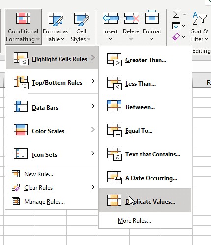
2. Access Conditional Formatting: Go to the “Home” tab, click “Conditional Formatting,” and then select “Highlight Cells Rules” followed by “Duplicate Values.”

3. Choose Formatting Style: A dialog box will appear, allowing you to choose the formatting style for duplicate values (e.g., light red fill with dark red text).
4. Apply Formatting: Click “OK” to apply the formatting. Excel will automatically highlight all duplicate entries in the selected range.

Advantages:

• Easy to implement.
• Provides a visual representation of duplicate values.
• No formulas required.

Disadvantages:

• Only highlights duplicates; it does not remove them.
• May not be suitable for large datasets due to performance considerations.

2.2 Utilizing the COUNTIF Function

The COUNTIF function counts the number of cells within a range that meet a given criterion. This function can be used to identify duplicates by counting how many times each value appears in a column.

1. Add a Helper Column: Insert a new column next to the column you want to check for duplicates.
2. Enter the COUNTIF Formula: In the first cell of the helper column, enter the COUNTIF formula: =COUNTIF($A:$A, A1) (assuming your data starts in column A).

3. Apply the Formula: Drag the formula down to apply it to all rows in your dataset. The helper column will now show the number of times each value appears in column A.
4. Filter for Duplicates: Use the filter option to display only rows where the COUNTIF value is greater than 1, indicating duplicate entries.

Advantages:

• Provides a count of how many times each value appears.
• Allows for easy filtering and identification of duplicates.
• Suitable for identifying duplicates based on specific criteria.

Disadvantages:

• Requires an additional helper column.
• May be slower for very large datasets.

2.3 Employing the EXACT Function

The EXACT function compares two strings and returns TRUE if they are exactly the same (case-sensitive), and FALSE otherwise. This function is useful for identifying duplicates where case sensitivity is important.

1. Add a Helper Column: Insert a new column next to the columns you want to compare.
2. Enter the EXACT Formula: In the first cell of the helper column, enter the EXACT formula: =EXACT(A1, B1) (assuming your data is in columns A and B).

3. Apply the Formula: Drag the formula down to apply it to all rows. The helper column will display TRUE for rows where the values in columns A and B are exactly the same, and FALSE otherwise.
4. Filter for Matches: Use the filter option to display only rows where the EXACT value is TRUE, indicating exact matches.

Advantages:

• Case-sensitive comparison.
• Useful for ensuring exact matches between two columns.

Disadvantages:

• Requires an additional helper column.
• Only compares two columns at a time.
• Case sensitivity may not be desirable in all scenarios.

2.4 Utilizing Advanced Filter

Excel’s advanced filter feature can be used to extract unique records from a dataset, effectively identifying and removing duplicates.

1. Select the Data Range: Select the range of cells you want to filter for duplicates.

2. Open Advanced Filter: Go to the “Data” tab and click “Advanced” in the “Sort & Filter” group.

3. Configure the Filter:

   • Choose “Copy to another location.”
   • Set the “List range” to your data range.
   • Set the “Criteria range” to an empty cell (this is required but not used in this case).
   • Set the “Copy to” location to a new cell where you want the unique records to be placed.
   • Check the “Unique records only” box.

4. Apply the Filter: Click “OK” to apply the filter. Excel will copy the unique records to the specified location, effectively removing duplicates from the output.

Advantages:

• Quickly extracts unique records.
• Does not require formulas or helper columns.
• Suitable for large datasets.

Disadvantages:

• Removes duplicates entirely, which may not be desirable in all cases.
• Requires copying the unique records to a new location.

2.5 Removing Duplicates Using the “Remove Duplicates” Feature

Excel’s built-in “Remove Duplicates” feature provides a straightforward way to eliminate duplicate rows based on selected columns.

1. Select the Data Range: Select the range of cells from which you want to remove duplicates.

2. Open Remove Duplicates: Go to the “Data” tab and click “Remove Duplicates” in the “Data Tools” group.

3. Select Columns to Check: A dialog box will appear, allowing you to select the columns you want to include in the duplicate check.

4. Remove Duplicates: Click “OK” to remove the duplicates. Excel will display a message indicating how many duplicate rows were removed.

Advantages:

• Simple and easy to use.
• Removes duplicates directly from the dataset.
• Allows selection of specific columns for the duplicate check.

Disadvantages:

• Permanently removes duplicates, which may not be desirable in all cases.
• May not be suitable for complex duplicate identification scenarios.

3. Step-by-Step Guides for Duplicate Comparison

How to compare duplicates in Excel using step-by-step guides? To effectively compare duplicates in Excel, detailed, step-by-step instructions are crucial. These guides provide clear, actionable steps for each method, ensuring users can confidently apply the techniques to their own datasets.

3.1 Conditional Formatting Step-by-Step

1. Open Your Excel Worksheet: Launch Microsoft Excel and open the worksheet containing the data you want to analyze.

2. Select the Data Range: Click and drag your mouse to select the range of cells you wish to check for duplicates. Make sure to include all relevant columns and rows.

3. Navigate to Conditional Formatting:

   • Go to the “Home” tab in the Excel ribbon.
   • In the “Styles” group, click on “Conditional Formatting.”

4. Choose Highlight Cells Rules:

   • In the dropdown menu, select “Highlight Cells Rules.”
   • Choose “Duplicate Values” from the submenu.

5. Configure Duplicate Values Formatting:

   • A dialog box will appear, allowing you to customize the formatting for duplicate values.

   • In the dropdown menu next to “with,” select the formatting style you prefer (e.g., “Light Red Fill with Dark Red Text”).

   • Click “OK” to apply the formatting.

6. Review Highlighted Duplicates:

   • Excel will now highlight all duplicate entries in the selected range according to the formatting style you chose.
   • Review the highlighted cells to identify duplicate records.

7. Optional: Customize Formatting:

   • If you want to change the formatting style, repeat steps 3-5 and choose a different style.
   • To remove the conditional formatting, go to “Conditional Formatting,” select “Clear Rules,” and choose “Clear Rules from Selected Cells.”

3.2 COUNTIF Function Step-by-Step

1. Open Your Excel Worksheet: Open the Excel worksheet that contains the data.

2. Insert a Helper Column:

   • Click on the column header next to the column you want to check for duplicates (e.g., if your data is in column A, click on column B).
   • Right-click and select “Insert” to add a new column.
   • Label the new column (e.g., “Duplicate Count”).

3. Enter the COUNTIF Formula:

   • In the first cell of the helper column (e.g., B1), enter the COUNTIF formula: =COUNTIF($A:$A, A1).
   • This formula counts how many times the value in cell A1 appears in column A.

4. Apply the Formula to All Rows:

   • Click on the cell with the COUNTIF formula (e.g., B1).
   • Hover your mouse over the bottom-right corner of the cell until you see a small black cross (+).
   • Double-click the cross to automatically apply the formula to all rows in the column.

5. Filter for Duplicates:

   • Select the header row of your data range.
   • Go to the “Data” tab and click on “Filter” in the “Sort & Filter” group.
   • Click the filter arrow in the helper column (e.g., column B).
   • Choose “Number Filters” and then select “Greater Than.”
   • Enter “1” in the dialog box and click “OK.” This will display only the rows where the COUNTIF value is greater than 1, indicating duplicate entries.

6. Review Filtered Duplicates:

   • Excel will now display only the duplicate entries.
   • Review the filtered rows to identify and manage duplicate records.

7. Optional: Remove Filter:

   • To remove the filter and display all rows, click the filter arrow in the helper column and select “Clear Filter From ‘Duplicate Count’.”

3.3 EXACT Function Step-by-Step

1. Open Your Excel Worksheet: Launch Excel and open the worksheet containing the data you want to compare.

2. Insert a Helper Column:

   • Click on the column header next to the columns you want to compare (e.g., if your data is in columns A and B, click on column C).
   • Right-click and select “Insert” to add a new column.
   • Label the new column (e.g., “Exact Match”).

3. Enter the EXACT Formula:

   • In the first cell of the helper column (e.g., C1), enter the EXACT formula: =EXACT(A1, B1).
   • This formula compares the values in cell A1 and cell B1 and returns TRUE if they are exactly the same (case-sensitive), and FALSE otherwise.

4. Apply the Formula to All Rows:

   • Click on the cell with the EXACT formula (e.g., C1).
   • Hover your mouse over the bottom-right corner of the cell until you see a small black cross (+).
   • Double-click the cross to automatically apply the formula to all rows in the column.

5. Filter for Matches:

   • Select the header row of your data range.
   • Go to the “Data” tab and click on “Filter” in the “Sort & Filter” group.
   • Click the filter arrow in the helper column (e.g., column C).
   • Uncheck “FALSE” to display only the rows where the values in columns A and B are exactly the same.
   • Click “OK.”

6. Review Filtered Matches:

   • Excel will now display only the rows where the values in columns A and B are exact matches.
   • Review the filtered rows to identify and manage matching records.

7. Optional: Remove Filter:

   • To remove the filter and display all rows, click the filter arrow in the helper column and select “Clear Filter From ‘Exact Match’.”

3.4 Advanced Filter Step-by-Step

1. Open Your Excel Worksheet: Open the Excel worksheet that contains the data from which you want to extract unique records.

2. Select the Data Range: Click and drag your mouse to select the range of cells that contains the data. Include the column headers in your selection.

3. Open the Advanced Filter Dialog Box:

   • Go to the “Data” tab in the Excel ribbon.
   • In the “Sort & Filter” group, click on “Advanced.”

4. Configure the Advanced Filter:

   • In the Advanced Filter dialog box, choose “Copy to another location.”
   • Set the “List range” to your data range (this should already be selected).
   • Leave the “Criteria range” blank (you can select an empty cell if required).
   • Set the “Copy to” location by clicking in the “Copy to” box and then selecting a cell where you want the unique records to be placed.
   • Check the “Unique records only” box.

5. Apply the Filter:

   • Click “OK” to apply the filter.
   • Excel will copy the unique records from your data range to the specified “Copy to” location.

6. Review Unique Records:

   • Review the copied data to ensure that all duplicate entries have been removed.
   • The new range will contain only unique records from the original dataset.

3.5 Remove Duplicates Feature Step-by-Step

1. Open Your Excel Worksheet: Launch Microsoft Excel and open the worksheet containing the data you want to clean.

2. Select the Data Range: Click and drag your mouse to select the range of cells from which you want to remove duplicates. Make sure to include the column headers in your selection.

3. Open the Remove Duplicates Dialog Box:

   • Go to the “Data” tab in the Excel ribbon.
   • In the “Data Tools” group, click on “Remove Duplicates.”

4. Select Columns to Check for Duplicates:

   • A dialog box will appear, listing all the column headers in your selected data range.
   • Check the boxes next to the columns you want to include in the duplicate check. Excel will consider a row as a duplicate only if the values in all selected columns are the same.

5. Remove Duplicates:

   • Click “OK” to remove the duplicates.
   • Excel will display a message indicating how many duplicate rows were found and removed, as well as how many unique rows remain.

6. Review Results:

   • Review your data to ensure that the duplicates have been removed and that the remaining data is accurate.
   • Note that the “Remove Duplicates” feature permanently deletes the duplicate rows, so it’s a good idea to save a backup of your data before using this feature.

4. Advanced Techniques for Comparing Duplicates

Beyond the basic methods, what are the advanced techniques for comparing duplicates? Excel offers advanced techniques that provide more flexibility and precision in identifying and managing duplicates. These techniques include using array formulas, combining multiple functions, and leveraging VBA scripts for custom solutions.

4.1 Using Array Formulas for Complex Comparisons

Array formulas allow you to perform complex calculations on entire arrays of data, making them useful for advanced duplicate comparisons. For example, you can use an array formula to compare two columns and return a list of unique values.

1. Enter the Array Formula: In a new column, enter the following array formula:
   =IFERROR(INDEX($A$1:$A$10, MATCH(0,COUNTIF($C$1:C1, $A$1:$A$10), 0)), "")
   • This formula assumes your data is in column A, and you are entering the formula in column C.
   • Press Ctrl + Shift + Enter to enter the formula as an array formula. Excel will automatically add curly braces {} around the formula.
2. Apply the Formula: Drag the formula down to apply it to all rows. The column will now display a list of unique values from column A.

Advantages:

• Allows for complex comparisons and calculations.
• Can return a list of unique values from a dataset.

Disadvantages:

• Can be difficult to understand and implement.
• May slow down Excel performance, especially for large datasets.

4.2 Combining Multiple Functions for Enhanced Accuracy

Combining multiple Excel functions can enhance the accuracy of duplicate comparisons by allowing you to create more specific criteria for identifying duplicates. For example, you can combine the TRIM and EXACT functions to compare two columns while ignoring leading and trailing spaces.

1. Add a Helper Column: Insert a new column next to the columns you want to compare.
2. Enter the Combined Formula: In the first cell of the helper column, enter the following formula:
   =EXACT(TRIM(A1), TRIM(B1))
   • This formula first trims any leading or trailing spaces from the values in cells A1 and B1, and then compares them using the EXACT function.
3. Apply the Formula: Drag the formula down to apply it to all rows. The helper column will display TRUE for rows where the trimmed values in columns A and B are exactly the same, and FALSE otherwise.

Advantages:

• Allows for more specific duplicate identification criteria.
• Can handle inconsistencies such as leading and trailing spaces.

Disadvantages:

• Requires a good understanding of Excel functions.
• Can become complex for very specific comparison scenarios.

4.3 Using VBA Scripts for Custom Solutions

VBA (Visual Basic for Applications) allows you to create custom scripts to automate tasks in Excel, including duplicate comparisons. You can write a VBA script to compare two columns and highlight or remove duplicates based on specific criteria.

1. Open the VBA Editor:
   • Press Alt + F11 to open the VBA editor in Excel.
2. Insert a New Module:
   • Go to “Insert” > “Module” to insert a new module.
3. Write the VBA Script:
   • Copy and paste the following VBA script into the module:

Sub CompareColumns()
    Dim ws As Worksheet
    Dim lastRow As Long
    Dim i As Long
    Dim j As Long

    Set ws = ThisWorkbook.Sheets("Sheet1") ' Change "Sheet1" to your sheet name
    lastRow = ws.Cells(Rows.Count, "A").End(xlUp).Row ' Assumes data starts in column A

    For i = 1 To lastRow
        For j = i + 1 To lastRow
            If ws.Cells(i, "A").Value = ws.Cells(j, "A").Value And _
               ws.Cells(i, "B").Value = ws.Cells(j, "B").Value Then ' Adjust columns as needed
                ws.Cells(i, "A").Interior.Color = RGB(255, 0, 0) ' Highlight duplicate in red
                ws.Cells(j, "A").Interior.Color = RGB(255, 0, 0)
            End If
        Next j
    Next i
End Sub

• This script compares values in columns A and B and highlights duplicates in red.
• Adjust the column letters and sheet name as needed.

4. Run the Script:
   • Close the VBA editor and go back to your Excel worksheet.
   • Go to the “Developer” tab and click “Macros.”
   • Select the CompareColumns macro and click “Run.”

Advantages:

• Provides maximum flexibility for custom duplicate comparison scenarios.
• Can automate complex tasks.

Disadvantages:

• Requires knowledge of VBA programming.
• Can be time-consuming to develop and debug.
• Macros must be enabled in Excel for the script to run.

5. Best Practices for Managing Duplicates in Excel

What are the best practices for managing duplicates in Excel? Managing duplicates effectively requires a combination of appropriate techniques, careful planning, and consistent execution. Following best practices ensures data integrity, enhances analysis accuracy, and streamlines spreadsheet management.

5.1 Regular Data Cleansing

Regular data cleansing is essential for maintaining high data quality. Schedule periodic reviews of your datasets to identify and remove duplicates, correct errors, and update outdated information. This proactive approach prevents data inconsistencies from accumulating and ensures that your analyses are based on accurate and reliable data.

5.2 Data Validation Techniques

Data validation helps prevent duplicates from being entered into your spreadsheet in the first place. Excel’s data validation feature allows you to set rules that restrict the type of data that can be entered into a cell, such as ensuring that all entries in a column are unique.

1. Select the Range: Select the cells where you want to apply data validation.
2. Open Data Validation: Go to the “Data” tab and click “Data Validation” in the “Data Tools” group.
3. Set Validation Criteria:
   • In the Data Validation dialog box, go to the “Settings” tab.
   • In the “Allow” dropdown menu, select “Custom.”
   • Enter the following formula in the “Formula” box:
     =COUNTIF($A:$A, A1)=1
     • This formula ensures that the value entered in the cell is unique in column A.
4. Set Error Alert:
   • Go to the “Error Alert” tab.
   • Check the “Show error alert after invalid data is entered” box.
   • Enter an appropriate title and error message (e.g., “Duplicate Entry” and “This value already exists. Please enter a unique value.”).
5. Apply Data Validation: Click “OK” to apply the data validation. Excel will now display an error message if you try to enter a duplicate value in the selected range.

5.3 Using Excel Tables for Improved Data Management

Excel tables provide enhanced data management features, including automatic expansion, structured references, and built-in filtering and sorting capabilities. Converting your data range to an Excel table simplifies duplicate management and improves overall data organization.

1. Select the Data Range: Select the range of cells you want to convert to a table.
2. Create the Table: Go to the “Insert” tab and click “Table” in the “Tables” group.
3. Confirm Table Range: In the Create Table dialog box, confirm that the selected range is correct and check the “My table has headers” box if your data includes column headers.
4. Apply Table Formatting: Click “OK” to create the table. Excel will automatically apply table formatting and enable table features.

5.4 Training and Documentation

Ensure that all users who work with your spreadsheets are trained on the proper techniques for managing duplicates. Provide clear documentation outlining the methods and best practices for identifying and removing duplicates, as well as the importance of maintaining data integrity.

6. Real-World Examples of Duplicate Comparison

How to compare duplicates in Excel in real-world examples? Examining real-world examples illustrates the practical applications of duplicate comparison in various industries and scenarios. These examples demonstrate how different techniques can be applied to solve specific data management challenges.

6.1 CRM Data Management

A marketing team uses Excel to manage customer data, including names, email addresses, and phone numbers. Over time, duplicate entries accumulate due to manual data entry errors and imports from various sources.

• Challenge: Identifying and removing duplicate customer records to avoid redundant marketing efforts and improve customer engagement.
• Solution:
  1. Use the “Remove Duplicates” feature to eliminate duplicate records based on email addresses and phone numbers.
  2. Implement data validation to prevent duplicate entries during manual data entry.
  3. Regularly cleanse the data to identify and merge similar records (e.g., different spellings of the same name).
• Outcome: Improved data accuracy, reduced marketing costs, and enhanced customer satisfaction.

6.2 Inventory Management

A retail company uses Excel to track inventory levels, including product names, SKUs, and quantities. Duplicate entries can lead to inaccurate stock counts and ordering errors.

• Challenge: Ensuring accurate stock levels by identifying and removing duplicate entries for products.
• Solution:
  1. Use the COUNTIF function to identify duplicate SKUs.
  2. Use conditional formatting to highlight duplicate product names.
  3. Implement data validation to ensure that all SKUs are unique.
• Outcome: Accurate inventory tracking, reduced ordering errors, and improved supply chain efficiency.

6.3 Financial Data Analysis

An accounting firm uses Excel to analyze financial transactions, including dates, amounts, and descriptions. Duplicate transactions can skew financial reports and lead to incorrect conclusions.

• Challenge: Eliminating duplicate transactions in financial records to ensure accurate accounting and reporting.
• Solution:
  1. Use the “Remove Duplicates” feature to eliminate duplicate transactions based on dates, amounts, and descriptions.
  2. Use the EXACT function to compare transaction descriptions for case-sensitive matches.
  3. Implement data validation to prevent duplicate entries during manual data entry.
• Outcome: Accurate financial reports, reliable audit trails, and improved financial decision-making.

7. Troubleshooting Common Issues

What are common issues and troubleshooting when you compare duplicates? Despite the effectiveness of Excel’s duplicate comparison tools, users may encounter common issues. Understanding these issues and how to troubleshoot them ensures a smooth and accurate duplicate management process.

7.1 False Positives

False positives occur when Excel identifies entries as duplicates that are actually unique. This can happen due to subtle differences in data, such as leading or trailing spaces, case sensitivity, or inconsistent formatting.

• Solution:
  1. Use the TRIM function to remove leading and trailing spaces.
  2. Use the EXACT function for case-sensitive comparisons.
  3. Ensure consistent formatting across all entries.
  4. Manually review highlighted duplicates to confirm their accuracy.

7.2 Performance Issues with Large Datasets

Comparing duplicates in very large datasets can slow down Excel’s performance, especially when using complex formulas or conditional formatting.

• Solution:
  1. Use the “Remove Duplicates” feature, which is optimized for large datasets.
  2. Disable automatic calculations and enable manual calculations.
  3. Use Excel tables to improve data management and performance.
  4. Break the data into smaller chunks and process them separately.

7.3 Incorrect Formula Results

Incorrect formula results can occur due to errors in the formula syntax, incorrect cell references, or logical errors in the comparison criteria.

• Solution:
  1. Double-check the formula syntax for errors.
  2. Ensure that cell references are correct and absolute references are used where necessary.
  3. Test the formula on a small subset of data to verify its accuracy.
  4. Use Excel’s formula auditing tools to trace errors and identify dependencies.

7.4 Data Validation Not Working

Data validation may not work if the validation rules are not set correctly or if existing data violates the validation rules.

• Solution:
  1. Double-check the data validation criteria and ensure that they are set correctly.
  2. Apply data validation to a clean dataset to prevent conflicts with existing data.
  3. Use the “Circle Invalid Data” feature to identify and correct existing data that violates the validation rules.
  4. Clear existing validation rules and reapply them to ensure they are properly enforced.

8. Conclusion: Mastering Duplicate Comparison in Excel

In conclusion, mastering how to compare duplicates in Excel is crucial for maintaining data integrity, enhancing analysis accuracy, and streamlining spreadsheet management. By understanding and applying the various techniques discussed in this guide, users can confidently identify and manage duplicate entries in their datasets. From basic methods like conditional formatting and the COUNTIF function to advanced techniques like array formulas and VBA scripts, Excel offers a range of tools to suit different scenarios and skill levels. Regular data cleansing, data validation, and the use of Excel tables further contribute to effective duplicate management.

Remember, accurate data leads to better decisions. Take the time to implement these best practices and transform your data management processes.

Ready to take your data management skills to the next level? Visit COMPARE.EDU.VN today to explore more in-depth guides, tutorials, and resources that will help you master Excel and other essential data analysis tools. Whether you’re a student, a professional, or simply someone who wants to make better decisions, COMPARE.EDU.VN is your go-to source for comprehensive comparisons and actionable insights. Start exploring now and unlock the full potential of your data!

Contact us:

• Address: 333 Comparison Plaza, Choice City, CA 90210, United States
• WhatsApp: +1 (626) 555-9090
• Website: compare.edu.vn

9. Frequently Asked Questions (FAQs)

9.1 How do I compare two columns in Excel for exact matches?

To compare two columns in Excel for exact matches, you can use the EXACT function. Enter the formula =EXACT(A1, B1) in a helper column to compare the values in cells A1 and B1. This function is case-sensitive and returns TRUE if the values are exactly the same, and FALSE otherwise. You can then filter the helper column to display only the rows where the values are exact matches.

9.2 Can I compare multiple columns for duplicates in Excel?

Yes, you can compare multiple columns for duplicates in Excel. One way to do this is by using the “Remove Duplicates” feature, which allows you to select multiple columns to check for duplicates. Excel will consider a row as a duplicate only if the values in all selected columns are the same. Alternatively, you can use a combination of functions like CONCATENATE and COUNTIF to compare multiple columns for duplicates.

9.3 How do I highlight duplicate rows in Excel?

To highlight duplicate rows in Excel, you can use conditional formatting. Select the range of cells you want to check for duplicates, go to the “Home” tab, click “Conditional Formatting,” and then select “Highlight Cells Rules” followed by “Duplicate Values.” Choose the formatting style you prefer and click “OK” to apply the formatting. Excel will automatically highlight all duplicate rows in the selected range.

9.4 How do I remove duplicates in Excel without losing data?

When removing duplicates in Excel, it’s a good practice to create a backup of your data before using the “Remove Duplicates” feature, as this feature permanently deletes the duplicate rows. Copy your data to another sheet before using this function.

9.5 How can I prevent duplicate entries in Excel?

You can prevent duplicate entries in Excel by using the data validation feature. Select the cells where you want to apply data validation, go to the “Data” tab, and click “Data Validation.” Set the validation criteria to ensure that the values entered in the cell are unique. This can be done by using the custom validation setting and the formula =COUNTIF($A:$A, A1)=1.

9.6 What is the best way to compare two columns if one column has extra spaces?

If one column has extra spaces, the best way to compare two columns is to use the TRIM function in combination with the EXACT function. The TRIM function removes leading and trailing spaces from the values, ensuring that the comparison is accurate. The combined formula would be =EXACT(TRIM(A1), TRIM(B1)).

9.7 How do I use VBA to compare duplicates in Excel?

To use VBA to compare