Comparing different columns in Excel is a fundamental skill for data analysis, manipulation, and informed decision-making. At COMPARE.EDU.VN, we understand the importance of efficiently comparing data across columns, whether it’s identifying duplicate entries, spotting unique values, or performing complex row-by-row comparisons, we provide the tools and guidance to streamline this process. Discover the power of Excel with our comprehensive techniques for comparing columns using conditional formatting, formulas, and lookup functions, ensuring accuracy and saving valuable time.
1. Why Comparing Columns in Excel is Essential
Excel is a powerful tool for organizing and analyzing data. Comparing columns within Excel spreadsheets is crucial for various tasks, from ensuring data consistency to identifying trends and anomalies.
1.1 Data Validation and Quality Control
Comparing columns helps ensure data integrity by identifying inconsistencies and errors. This is particularly important when merging data from different sources or when tracking changes over time. For instance, if you have customer data in two columns, comparing them can help you identify duplicate entries or discrepancies in addresses.
1.2 Identifying Trends and Patterns
By comparing columns, you can uncover patterns and trends that might not be immediately obvious. This can be useful in a variety of fields, such as finance, marketing, and sales. For example, comparing sales data from different regions can help you identify which products are performing well in each area.
1.3 Making Informed Decisions
Ultimately, the goal of comparing columns in Excel is to make better decisions. By having a clear understanding of your data, you can make more informed choices about everything from resource allocation to product development. Imagine comparing projected sales figures with actual sales figures to adjust inventory and marketing strategies.
1.4 Use Cases for Comparing Columns
- Finance: Analyzing financial statements to identify discrepancies.
- Marketing: Comparing campaign performance across different channels.
- Sales: Tracking sales figures by region or product.
- Human Resources: Managing employee data and identifying missing information.
- Inventory Management: Matching inventory records with sales data to optimize stock levels.
2. Basic Techniques for Comparing Columns in Excel
Several basic techniques can be employed to compare columns in Excel, each offering its own advantages and use cases.
2.1 Using the Equals Operator
The simplest method for comparing two columns is using the equals operator (=). This method performs a row-by-row comparison and returns TRUE if the values in the two cells are identical, and FALSE otherwise.
2.1.1 How to Use the Equals Operator
- In a new column (e.g., Column D), enter the formula
=A1=B1in the first cell (D1). - Drag the fill handle (the small square at the bottom-right of the cell) down to apply the formula to all rows.
- Excel will display TRUE for matching rows and FALSE for non-matching rows.
2.1.2 Example
| Column A | Column B | Column C (Formula: =A1=B1) |
|---|---|---|
| Apple | Apple | TRUE |
| Banana | Orange | FALSE |
| Cherry | Cherry | TRUE |
2.2 Using the IF Function
The IF function allows you to display custom messages instead of TRUE or FALSE, making the comparison results more user-friendly.
2.2.1 How to Use the IF Function
- In a new column (e.g., Column D), enter the formula
=IF(A1=B1, "Match", "No Match")in the first cell (D1). - Drag the fill handle down to apply the formula to all rows.
- Excel will display “Match” for matching rows and “No Match” for non-matching rows.
2.2.2 Example
| Column A | Column B | Column C (Formula: =IF(A1=B1, “Match”, “No Match”)) |
|---|---|---|
| Apple | Apple | Match |
| Banana | Orange | No Match |
| Cherry | Cherry | Match |
2.3 Using the EXACT Function
The EXACT function is case-sensitive, meaning it distinguishes between uppercase and lowercase letters. This is useful when you need to ensure that the values in the two columns are exactly the same.
2.3.1 How to Use the EXACT Function
- In a new column (e.g., Column D), enter the formula
=IF(EXACT(A1, B1), "Exact Match", "Not Exact")in the first cell (D1). - Drag the fill handle down to apply the formula to all rows.
- Excel will display “Exact Match” for rows where the values are identical, including case, and “Not Exact” otherwise.
2.3.2 Example
| Column A | Column B | Column C (Formula: =IF(EXACT(A1, B1), “Exact Match”, “Not Exact”)) |
|---|---|---|
| Apple | Apple | Exact Match |
| Apple | apple | Not Exact |
| Cherry | Cherry | Exact Match |
3. Advanced Techniques for Comparing Columns in Excel
For more complex comparisons, Excel offers advanced techniques that provide greater flexibility and control.
3.1 Conditional Formatting
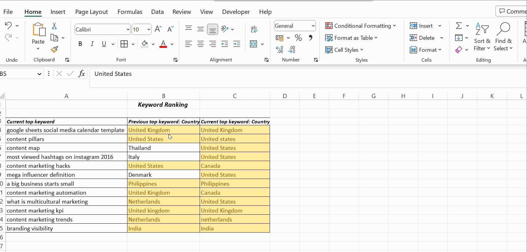
Conditional formatting allows you to highlight cells based on certain criteria. This can be used to visually identify matching or non-matching values in two columns.
3.1.1 How to Use Conditional Formatting
- Select the range of cells you want to compare (e.g., Columns A and B).
- Go to Home > Conditional Formatting > New Rule.
- Select “Use a formula to determine which cells to format”.
- Enter the formula
=A1=B1in the formula box. - Click Format and choose a fill color or other formatting options to highlight matching cells.
- Click OK to apply the rule.
- Repeat the process to create a second rule with the formula
=A1<>B1to highlight non-matching cells with a different format.
3.1.2 Example
By setting up conditional formatting, you can quickly see which cells in Columns A and B match (e.g., highlighted in green) and which do not (e.g., highlighted in red).
3.2 Using Lookup Functions (VLOOKUP, HLOOKUP, XLOOKUP)
Lookup functions such as VLOOKUP, HLOOKUP, and XLOOKUP are useful for comparing columns based on a lookup value. These functions search for a value in one column and return a corresponding value from another column.
3.2.1 VLOOKUP (Vertical Lookup)
VLOOKUP searches for a value in the first column of a range and returns a value from a specified column in the same row.
How to Use VLOOKUP
- Suppose you have a list of product IDs in Column A and a list of product names in Column B. You want to compare this list with a second list of product IDs in Column C and retrieve the corresponding product names from Column B.
- In Column D, enter the formula
=VLOOKUP(C1, A:B, 2, FALSE)in the first cell (D1). - Drag the fill handle down to apply the formula to all rows.
- Excel will display the product name from Column B if the product ID in Column C is found in Column A. If the product ID is not found, it will display #N/A.
Example
| Column A (Product ID) | Column B (Product Name) | Column C (Product ID) | Column D (Formula: =VLOOKUP(C1, A:B, 2, FALSE)) |
|---|---|---|---|
| 101 | Apple | 101 | Apple |
| 102 | Banana | 103 | #N/A |
| 103 | Cherry | 102 | Banana |
3.2.2 HLOOKUP (Horizontal Lookup)
HLOOKUP searches for a value in the first row of a range and returns a value from a specified row in the same column.
How to Use HLOOKUP
- HLOOKUP is used similarly to VLOOKUP, but for horizontal data. For example, if your product IDs and names are arranged in rows instead of columns, you would use HLOOKUP.
- Enter the formula
=HLOOKUP(C1, A1:B2, 2, FALSE)in the appropriate cell.
3.2.3 XLOOKUP
XLOOKUP is a more versatile lookup function that can search in both vertical and horizontal ranges. It also offers improved error handling and performance.
How to Use XLOOKUP
- Using the same example as VLOOKUP, enter the formula
=XLOOKUP(C1, A:A, B:B, "Not Found")in Column D. - Drag the fill handle down to apply the formula to all rows.
- Excel will display the product name from Column B if the product ID in Column C is found in Column A. If the product ID is not found, it will display “Not Found”.
Example
| Column A (Product ID) | Column B (Product Name) | Column C (Product ID) | Column D (Formula: =XLOOKUP(C1, A:A, B:B, “Not Found”)) |
|---|---|---|---|
| 101 | Apple | 101 | Apple |
| 102 | Banana | 103 | Not Found |
| 103 | Cherry | 102 | Banana |
3.3 Combining Functions for Complex Comparisons
You can combine multiple functions to perform more complex comparisons. For example, you can use the IF function along with the AND or OR functions to check multiple conditions.
3.3.1 Using IF with AND
The AND function checks if all conditions are true.
How to Use IF with AND
- Suppose you want to check if both the product ID and product name match between two lists.
- In a new column, enter the formula
=IF(AND(A1=C1, B1=D1), "Match", "No Match"). - Drag the fill handle down to apply the formula to all rows.
- Excel will display “Match” only if both the product ID and product name match in the corresponding rows.
Example
| Column A (Product ID) | Column B (Product Name) | Column C (Product ID) | Column D (Product Name) | Column E (Formula: =IF(AND(A1=C1, B1=D1), “Match”, “No Match”)) |
|---|---|---|---|---|
| 101 | Apple | 101 | Apple | Match |
| 102 | Banana | 102 | Orange | No Match |
| 103 | Cherry | 103 | Cherry | Match |
3.3.2 Using IF with OR
The OR function checks if at least one condition is true.
How to Use IF with OR
- Suppose you want to check if either the product ID or product name matches between two lists.
- In a new column, enter the formula
=IF(OR(A1=C1, B1=D1), "Partial Match", "No Match"). - Drag the fill handle down to apply the formula to all rows.
- Excel will display “Partial Match” if either the product ID or product name matches in the corresponding rows.
Example
| Column A (Product ID) | Column B (Product Name) | Column C (Product ID) | Column D (Product Name) | Column E (Formula: =IF(OR(A1=C1, B1=D1), “Partial Match”, “No Match”)) |
|---|---|---|---|---|
| 101 | Apple | 101 | Apple | Partial Match |
| 102 | Banana | 102 | Orange | Partial Match |
| 103 | Cherry | 104 | Cherry | Partial Match |
3.4 Using Array Formulas
Array formulas allow you to perform calculations on multiple values at once. This can be useful for comparing entire columns or ranges of cells.
3.4.1 How to Use Array Formulas
- Suppose you want to count the number of matching rows between two columns.
- Select a cell where you want to display the result.
- Enter the formula
=SUM(IF(A1:A10=B1:B10, 1, 0))and press Ctrl + Shift + Enter to enter it as an array formula. - Excel will display the number of matching rows between Columns A and B.
3.4.2 Example
| Column A | Column B |
|---|---|
| Apple | Apple |
| Banana | Orange |
| Cherry | Cherry |
| Apple | Banana |
| Orange | Orange |
The array formula =SUM(IF(A1:A5=B1:B5, 1, 0)) will return 3, as there are three matching rows.
4. Practical Examples of Comparing Columns
Let’s explore some practical examples of how to compare columns in Excel in different scenarios.
4.1 Comparing Customer Lists
Suppose you have two customer lists and want to identify duplicate entries.
4.1.1 Scenario
- Column A: Customer IDs from List 1
- Column B: Customer IDs from List 2
4.1.2 Solution
- In Column C, enter the formula
=IF(ISNUMBER(MATCH(A1, B:B, 0)), "Duplicate", ""). - Drag the fill handle down to apply the formula to all rows in Column A.
- Excel will display “Duplicate” for customer IDs that appear in both lists.
4.1.3 Explanation
- The
MATCHfunction searches for the value in A1 within the entire Column B. If a match is found, it returns the position of the match; otherwise, it returns an error. - The
ISNUMBERfunction checks if the result of theMATCHfunction is a number (i.e., a match was found). - The
IFfunction displays “Duplicate” if a match is found and leaves the cell blank otherwise.
4.2 Comparing Sales Data
Suppose you want to compare sales data for different products across two months.
4.2.1 Scenario
- Column A: Product Names
- Column B: Sales in January
- Column C: Sales in February
4.2.2 Solution
- In Column D, enter the formula
=C1-B1to calculate the difference in sales between February and January. - Drag the fill handle down to apply the formula to all rows.
- Format Column D to display the values as currency.
- Use conditional formatting to highlight products with significant increases or decreases in sales.
4.2.3 Explanation
- The formula
C1-B1calculates the difference between the sales in February (Column C) and January (Column B). - Conditional formatting can be used to highlight cells in Column D based on certain criteria, such as:
- Highlight cells with values greater than a certain threshold (e.g., $1000) in green to indicate significant increases in sales.
- Highlight cells with values less than a certain threshold (e.g., -$1000) in red to indicate significant decreases in sales.
4.3 Comparing Inventory Records
Suppose you want to compare inventory records with sales data to identify discrepancies.
4.3.1 Scenario
- Column A: Product IDs
- Column B: Quantity in Stock
- Column C: Quantity Sold
4.3.2 Solution
- In Column D, enter the formula
=B1-C1to calculate the remaining quantity in stock after sales. - Drag the fill handle down to apply the formula to all rows.
- Use conditional formatting to highlight products with negative remaining quantities, indicating potential discrepancies.
4.3.3 Explanation
- The formula
B1-C1calculates the difference between the quantity in stock (Column B) and the quantity sold (Column C). - Conditional formatting can be used to highlight cells in Column D with negative values, indicating that more products were sold than were in stock.
5. Tips for Efficient Column Comparison
To ensure accurate and efficient column comparison, consider the following tips.
5.1 Clean Your Data First
Before comparing columns, ensure that your data is clean and consistent. This includes:
- Removing any leading or trailing spaces using the
TRIMfunction. - Standardizing text case using the
UPPER,LOWER, orPROPERfunctions. - Converting data types to ensure that values are comparable (e.g., converting text to numbers).
5.2 Use Absolute References
When using formulas that involve ranges of cells, use absolute references (e.g., $A$1:$B$10) to prevent the range from changing when you drag the fill handle down.
5.3 Test Your Formulas
Before applying a formula to an entire column, test it on a few rows to ensure that it is working correctly.
5.4 Use Comments
Add comments to your formulas to explain what they do. This will make it easier for you and others to understand the formulas later.
5.5 Leverage Excel Tables
Convert your data ranges into Excel tables to take advantage of features such as:
- Automatic formula propagation: When you add a new row to a table, formulas are automatically applied to the new row.
- Structured references: Use table and column names in your formulas instead of cell references.
- Filtering and sorting: Easily filter and sort your data based on different criteria.
6. Troubleshooting Common Issues
When comparing columns in Excel, you may encounter some common issues. Here are some tips for troubleshooting them.
6.1 Formulas Not Working
If your formulas are not working correctly, check the following:
- Make sure that you have entered the formula correctly.
- Check that the cell references are correct.
- Ensure that the data types are compatible.
6.2 Incorrect Results
If your formulas are returning incorrect results, check the following:
- Make sure that you are using the correct formula for the comparison you want to perform.
- Check that your data is clean and consistent.
- Test your formula on a few rows to see if it is working as expected.
6.3 Performance Issues
If you are working with large datasets, you may experience performance issues. Here are some tips for improving performance:
- Use array formulas sparingly, as they can be resource-intensive.
- Disable automatic calculations and manually calculate the worksheet when needed.
- Close any unnecessary workbooks or applications.
7. How COMPARE.EDU.VN Can Help
At COMPARE.EDU.VN, we understand the importance of efficient data comparison and decision-making. Our platform offers a range of resources to help you master Excel and other data analysis tools.
7.1 Comprehensive Comparison Guides
We provide detailed guides on comparing various products, services, and ideas, giving you the information you need to make informed decisions. Whether you’re comparing different software solutions or evaluating the features of various consumer products, our comparison guides offer clear, objective insights.
7.2 Expert Reviews and User Feedback
Our platform features expert reviews and user feedback to provide a balanced view of different options. This helps you understand the pros and cons of each choice, ensuring that you’re making the best decision for your needs.
7.3 Customizable Comparison Tables
COMPARE.EDU.VN allows you to create customizable comparison tables to evaluate different options side-by-side. This feature enables you to focus on the criteria that are most important to you, making the decision-making process more efficient and effective.
7.4 Access to Reliable Information
We gather information from trusted sources to ensure that our comparisons are accurate and up-to-date. This saves you time and effort in researching different options, giving you the confidence to make the right choice.
8. Excel Alternatives for Column Comparison
While Excel is a powerful tool, there are alternative software options that may be better suited for certain types of column comparisons.
8.1 Google Sheets
Google Sheets is a web-based spreadsheet program that offers similar functionality to Excel. It is a good option for collaboration, as multiple users can work on the same spreadsheet simultaneously.
8.1.1 Advantages
- Collaboration: Real-time collaboration with multiple users.
- Accessibility: Accessible from any device with an internet connection.
- Cost: Free for personal use.
8.1.2 Disadvantages
- Functionality: Fewer advanced features than Excel.
- Performance: May be slower with large datasets.
8.2 Python with Pandas
Python is a programming language that is widely used for data analysis. The Pandas library provides data structures and functions for working with structured data, making it a powerful tool for column comparison.
8.2.1 Advantages
- Flexibility: Highly customizable and suitable for complex data manipulations.
- Scalability: Can handle large datasets efficiently.
- Integration: Integrates well with other data analysis tools and libraries.
8.2.2 Disadvantages
- Learning Curve: Requires programming knowledge.
- Setup: Requires installation of Python and the Pandas library.
8.3 SQL (Structured Query Language)
SQL is a programming language used for managing and manipulating data in relational databases. It is a good option for comparing columns in large databases.
8.3.1 Advantages
- Efficiency: Optimized for querying and manipulating large datasets.
- Data Integrity: Ensures data consistency and integrity.
- Standardization: Widely used and supported across different database systems.
8.3.2 Disadvantages
- Complexity: Requires knowledge of SQL and database management.
- Setup: Requires a database system and SQL client.
9. Best Practices for Data Analysis in Excel
To maximize the effectiveness of your column comparisons and data analysis in Excel, follow these best practices.
9.1 Plan Your Analysis
Before you start comparing columns, take some time to plan your analysis. This includes:
- Defining your objectives: What do you want to achieve with your analysis?
- Identifying the data you need: What data do you need to compare?
- Choosing the right techniques: Which techniques are best suited for your analysis?
9.2 Document Your Work
Document your work as you go along. This includes:
- Adding comments to your formulas to explain what they do.
- Creating a log of the steps you have taken.
- Saving your work regularly.
9.3 Validate Your Results
Validate your results to ensure that they are accurate and reliable. This includes:
- Checking your formulas for errors.
- Comparing your results with other sources of information.
- Testing your results on a sample of your data.
9.4 Present Your Findings
Present your findings in a clear and concise manner. This includes:
- Using charts and graphs to visualize your data.
- Writing a summary of your findings.
- Making recommendations based on your analysis.
10. FAQs About Comparing Columns in Excel
10.1 How do I compare two columns in Excel for exact matches?
Use the EXACT function within an IF statement: =IF(EXACT(A1, B1), "Match", "No Match").
10.2 Can I compare columns in different Excel sheets?
Yes, reference the sheet name in your formula: =IF(Sheet1!A1=Sheet2!A1, "Match", "No Match").
10.3 How can I highlight differences between two columns?
Use conditional formatting with the formula =A1<>B1 to highlight differing cells.
10.4 Is there a way to compare three or more columns at once?
Use AND within an IF statement: =IF(AND(A1=B1, A1=C1), "Match", "No Match").
10.5 How do I ignore case when comparing columns?
Use the UPPER or LOWER functions to convert text to the same case before comparing: =IF(UPPER(A1)=UPPER(B1), "Match", "No Match").
10.6 What is the best way to find unique values in two columns?
Use the COUNTIF function: =IF(COUNTIF(B:B, A1)=0, "Unique", "") in column A.
10.7 How do I compare numbers in two columns and find the differences?
Subtract one column from the other: =A1-B1.
10.8 Can I use wildcards when comparing columns?
Yes, use functions like SEARCH or FIND within an IF statement: =IF(ISNUMBER(SEARCH("*text*", A1)), "Match", "No Match").
10.9 How do I compare dates in two columns?
Ensure both columns are formatted as dates and use the equals operator or subtraction.
10.10 How do I handle errors when comparing columns?
Use the IFERROR function to return a custom message when an error occurs: =IFERROR(VLOOKUP(A1, B:C, 2, FALSE), "Not Found").
Conclusion
Comparing different columns in Excel is a fundamental skill for data analysis, enabling you to validate data, identify trends, and make informed decisions. Whether you’re using basic techniques like the equals operator and IF function or advanced methods like conditional formatting and lookup functions, Excel offers a range of tools to streamline the comparison process. By following best practices and leveraging resources like COMPARE.EDU.VN, you can master column comparison and unlock the full potential of Excel for your data analysis needs.
Ready to take your Excel skills to the next level? Visit COMPARE.EDU.VN today to explore our comprehensive comparison guides, expert reviews, and customizable comparison tables. Make informed decisions with confidence and unlock the power of data analysis. For further assistance, contact us at 333 Comparison Plaza, Choice City, CA 90210, United States. Reach out via Whatsapp at +1 (626) 555-9090 or visit our website compare.edu.vn.