**How To Compare Data Of Two Columns In Excel: A Comprehensive Guide**

Unlock the power of Excel and learn How To Compare Data Of Two Columns In Excel effortlessly. This guide from COMPARE.EDU.VN provides a complete walkthrough of various methods, empowering you to identify matches, differences, and unique values with ease. Master Excel data comparison for insightful analysis.

Are you struggling to manually sift through endless rows of data in Excel, searching for matches, differences, or unique values between two columns? At COMPARE.EDU.VN, we understand this challenge. This article offers several effective strategies to compare data of two columns in Excel, ensuring accuracy and efficiency in your data analysis. Delve into conditional formatting, explore the versatility of the VLOOKUP function, and master the IF and EXACT formulas. Uncover the full potential of your spreadsheets with our step-by-step instructions and detailed explanations.

1. Understanding Data Comparison in Excel

What exactly does it mean to compare columns in Excel? Why is this such a crucial skill for data analysts and other professionals?

Comparing columns in Excel involves examining corresponding cells within two or more columns to identify similarities, differences, or unique entries. This process is fundamental to data validation, cleaning, and analysis. It allows you to:

• Identify duplicates: Pinpoint identical entries across columns.
• Find missing values: Determine which values are present in one column but absent in another.
• Verify data integrity: Ensure consistency between related datasets.
• Track changes: Monitor how data has evolved over time.

These capabilities are essential for various tasks, including:

• Data cleansing: Correcting inconsistencies and errors in your data.
• Reporting: Generating accurate and reliable reports based on validated data.
• Decision-making: Making informed decisions based on comprehensive data analysis.

2. Key Search Intents Addressed in This Guide

This comprehensive guide is designed to address the following key search intents related to comparing data in Excel:

1. “How to compare two columns in Excel for differences”: Find methods to identify discrepancies between two columns of data.
2. “Compare two columns in Excel for matches”: Discover techniques to locate identical entries in two columns.
3. “Excel compare two columns and return value”: Learn how to compare columns and retrieve corresponding values based on the comparison.
4. “Excel compare two columns and highlight differences”: Find methods to visually highlight the differences between two columns.
5. “Compare two columns in Excel formula”: Explore various Excel formulas used for comparing data in columns.

3. Methods for Comparing Two Columns in Excel

Excel offers multiple methods for comparing data in two columns, each with its own strengths and weaknesses. Here, we will delve into five effective techniques, providing step-by-step instructions and practical examples:

1. Conditional Formatting
2. Equals Operator (=)
3. VLOOKUP Function
4. IF Formula
5. EXACT Formula

Let’s explore each of these methods in detail.

3.1. Using Conditional Formatting in Excel

Conditional formatting is a quick and visual way to highlight differences or matches between two columns. Here’s how to use it:

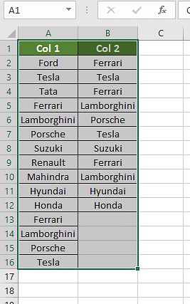
3.1.1. Step 1: Select the Data

First, select all the cells in the spreadsheet that you want to compare. Ensure that the columns you intend to compare are included in the selection.

3.1.2. Step 2: Access Conditional Formatting

Navigate to the “Home” tab on the Excel ribbon. In the “Styles” group, click on “Conditional Formatting.”

3.1.3. Step 3: Highlight Duplicate or Unique Values

A dropdown menu will appear. Choose “Highlight Cells Rules,” and then select either “Duplicate Values” or “Unique Values,” depending on what you want to identify.

3.1.3.1. Highlighting Duplicate Values

If you select “Duplicate Values,” Excel will open a new window. In this window, you can choose the formatting style for the duplicate values. The default is light red fill with dark red text, but you can customize it to your preference.

3.1.3.2. Highlighting Unique Values

If you choose “Unique Values,” a similar window will appear, allowing you to format the unique values. This is useful for identifying entries that exist in one column but not the other.

3.1.4. Step 4: Customize the Formatting (Optional)

In the formatting window, you can customize the fill color, font color, font style, and other formatting options to make the highlighted values more visible.

3.1.5. Step 5: Apply the Formatting

Click “OK” to apply the conditional formatting rule. Excel will now highlight the duplicate or unique values in your selected columns based on the criteria you specified.

3.2. Using the Equals Operator (=) to Compare Columns

The equals operator (=) provides a straightforward way to compare individual cells in two columns and return a TRUE or FALSE value indicating whether they match.

3.2.1. Step 1: Create a Result Column

Insert a new column next to the columns you want to compare. This column will display the results of the comparison.

3.2.2. Step 2: Enter the Formula

In the first cell of the result column, enter the following formula:

=A2=B2

Replace “A2” and “B2” with the cell addresses of the first cells you want to compare in each column.

3.2.3. Step 3: Apply the Formula to the Entire Column

Drag the fill handle (the small square at the bottom-right corner of the cell) down to apply the formula to all the rows in your data.

Excel will display “TRUE” for rows where the corresponding cells in the two columns match and “FALSE” for rows where they differ.

3.2.4. Step 4: Customize the Output (Optional)

You can use the IF function to display custom messages instead of “TRUE” and “FALSE.” For example:

=IF(A2=B2, "Match", "No Match")

This formula will display “Match” if the cells are identical and “No Match” if they are different.

3.3. Utilizing the VLOOKUP Function for Column Comparison

The VLOOKUP function is a powerful tool for comparing two columns and retrieving corresponding values from one column based on matches in the other.

3.3.1. Understanding the VLOOKUP Syntax

The VLOOKUP function has the following syntax:

=VLOOKUP(lookup_value, table_array, col_index_num, [range_lookup])

• lookup_value: The value you want to search for in the first column of the table array.
• table_array: The range of cells that contains the data you want to search and retrieve.
• col_index_num: The column number within the table array that contains the value you want to retrieve.
• [range_lookup]: An optional argument that specifies whether you want an exact match (FALSE) or an approximate match (TRUE). It is generally recommended to use FALSE for exact matches when comparing columns.

3.3.2. Step 1: Create a Result Column

As with the equals operator method, create a new column to display the results of the VLOOKUP function.

3.3.3. Step 2: Enter the VLOOKUP Formula

In the first cell of the result column, enter the following formula:

=VLOOKUP(A2, B:B, 1, FALSE)

Replace “A2” with the cell address of the value you want to look up in the first column. “B:B” represents the entire column B, where you want to search for the lookup value. “1” indicates that you want to retrieve the value from the first column of the table array (in this case, column B itself). “FALSE” specifies that you want an exact match.

3.3.4. Step 3: Apply the Formula to the Entire Column

Drag the fill handle down to apply the formula to all the rows in your data.

If the VLOOKUP function finds a match, it will return the matching value from the second column. If it doesn’t find a match, it will return a “#N/A” error.

3.3.5. Step 4: Handle Errors (Optional)

To handle the “#N/A” errors, you can use the IFERROR function to display a custom message when a match is not found. For example:

=IFERROR(VLOOKUP(A2, B:B, 1, FALSE), "Not Found")

This formula will display “Not Found” if the VLOOKUP function doesn’t find a match.

3.3.6. Step 5: Applying Wildcards (Optional)

The VLOOKUP function can sometimes return “FALSE” even if both cells represent the same data due to slight variations, such as extra spaces or characters. In such cases, you can use wildcards to broaden the search criteria.

For example, if you are comparing “Ford India” in one column with “Ford” in another, the standard VLOOKUP might return “FALSE.” To avoid this, you can modify the formula to include wildcards:

=IFERROR(VLOOKUP(A2&"*", B:B, 1, FALSE), "Not Found")

The “&”*” adds a wildcard to the lookup value, allowing it to match values that contain the lookup value as a substring.

3.4. Comparing with the IF Formula

The IF formula allows you to specify a condition and return different values based on whether the condition is TRUE or FALSE. This is particularly useful for comparing two columns and displaying custom messages indicating whether the values match or differ.

3.4.1. Understanding the IF Formula Syntax

The IF formula has the following syntax:

=IF(condition, value_if_true, value_if_false)

• condition: The condition you want to evaluate.
• value_if_true: The value to return if the condition is TRUE.
• value_if_false: The value to return if the condition is FALSE.

3.4.2. Step 1: Create a Result Column

As with the previous methods, create a new column to display the results of the IF formula.

3.4.3. Step 2: Enter the IF Formula

In the first cell of the result column, enter the following formula:

=IF(A2=B2, "Match", "No Match")

Replace “A2” and “B2” with the cell addresses of the first cells you want to compare in each column. This formula will display “Match” if the values in the two cells are equal and “No Match” if they are different.

3.4.4. Step 3: Apply the Formula to the Entire Column

Drag the fill handle down to apply the formula to all the rows in your data.

Excel will now display “Match” or “No Match” in the result column based on whether the corresponding cells in the two columns match.

For instance, if you want the result to be “Different car brands” if the names of the brands do not match, and “Same car brands” if the names match, you can use the following formula:

=IF(A2=B2, "Same car brands", "Different car brands")

3.5. Utilizing the EXACT Formula for Case-Sensitive Comparisons

The EXACT formula compares two strings and returns TRUE if they are exactly the same, including case. This is useful when you need to ensure that the values in two columns match exactly, including capitalization.

3.5.1. Understanding the EXACT Formula Syntax

The EXACT formula has the following syntax:

=EXACT(text1, text2)

• text1: The first text string to compare.
• text2: The second text string to compare.

3.5.2. Step 1: Create a Result Column

Create a new column to display the results of the EXACT formula.

3.5.3. Step 2: Enter the EXACT Formula

In the first cell of the result column, enter the following formula:

=EXACT(A2, B2)

Replace “A2” and “B2” with the cell addresses of the first cells you want to compare in each column. This formula will return TRUE if the values in the two cells are exactly the same (including case) and FALSE if they are different.

3.5.4. Step 3: Apply the Formula to the Entire Column

Drag the fill handle down to apply the formula to all the rows in your data.

Excel will now display TRUE or FALSE in the result column based on whether the corresponding cells in the two columns match exactly.

It’s important to remember that the EXACT formula is case-sensitive. If you write “Honda” in two different cases (e.g., “Honda” and “honda”) and apply the formula “=EXACT(A12, B12),” you will get the result “FALSE.” However, if the case is the same in both cells, the result will be “TRUE.”

4. Choosing the Right Method for Your Scenario

With several methods available for comparing two columns in Excel, how do you decide which one is best for your specific needs? Here’s a guide to help you choose the right approach:

4.1. Comparing Two Columns Row-by-Row

If you need to compare two columns on a row-by-row basis, determining whether the values in each row match or differ, use the following formulas:

• =IF(A2=B2, “Match”, ” “): This formula returns “Match” if the values in cells A2 and B2 are equal and a blank space if they are not.
• =IF(A2<>B2, “No Match”, ” “): This formula returns “No Match” if the values in cells A2 and B2 are different and a blank space if they are equal.
• =IF(A2=B2, “Match”, “No Match”): This formula returns “Match” if the values in cells A2 and B2 are equal and “No Match” if they are different.

For case-sensitive comparisons, use the EXACT formula within the IF formula:

• =IF(EXACT(A2, B2), “Match”, ” “): This formula returns “Match” if the values in cells A2 and B2 are exactly the same (including case) and a blank space if they are not.
• =IF(EXACT(A2, B2), “Match”, “No Match”): This formula returns “Match” if the values in cells A2 and B2 are exactly the same (including case) and “No Match” if they are not.

4.2. Comparing Multiple Columns for Row Matches

If you need to compare more than two columns to find rows where all values match, use the following formulas:

• =IF(AND(A2=B2, A2=C2), “Complete Match”, ” “): This formula returns “Complete Match” if the values in cells A2, B2, and C2 are all equal and a blank space if they are not.
• =IF(COUNTIF($A2:$E2, $A2)=4, “Complete Match”, ” “): This formula returns “Complete Match” if the value in cell A2 appears 4 times in the range A2:E2 (meaning all 5 cells have the same value) and a blank space if it does not. Adjust the number 4 to match the number of columns you are comparing minus one.

To compare columns and identify rows where any two or more cells have the same values, use the following formulas:

• =IF(OR(A2=B2, B2=C2, A2=C2), “Match”, “”): This formula returns “Match” if any of the following conditions are true: A2=B2, B2=C2, or A2=C2.
• =IF(COUNTIF(B2:D2,A2)+COUNTIF(C2:D2,B2)+(C2=D2)=0,”Unique”,”Match”): This formula returns “Unique” if all three cells (A2, B2, and C2) have different values and “Match” if any two or more cells have the same value.

4.3. Comparing Two Columns for Matches and Differences

To compare two datasets and identify the unique values present in column A but not in column B, use the following formulas:

• =IF(COUNTIF($B:$B, $A2)=0, “Not present in B”, “”): This formula returns “Not present in B” if the value in cell A2 does not exist in column B and a blank space if it does.
• =IF(ISERROR(MATCH($A2,$B$2:$B$10,0)),”Not present in B”,””): This formula returns “Not present in B” if the value in cell A2 cannot be found in the range B2:B10 and a blank space if it can.

To get a single result indicating both matches and unique values, use the following formula:

• =IF(COUNTIF($B:$B, $A2)=0, “Not Present in B”, “Present in B”): This formula returns “Not Present in B” if the value in cell A2 does not exist in column B and “Present in B” if it does.

4.4. Comparing Two Lists and Pulling Matching Data

To compare two lists and find the matching data, you can use the VLOOKUP function. You can also use the INDEX MATCH or XLOOKUP functions. Here are the formulas for this scenario:

• =VLOOKUP(D2, $A$2:$B$6, 2, FALSE): This formula searches for the value in cell D2 within the range A2:A6 and returns the corresponding value from the second column (column B) of the range.
• =INDEX($B$2:$B$6, MATCH($D2, $A$2:$A$6, 0)): This formula searches for the value in cell D2 within the range A2:A6 and returns the corresponding value from the range B2:B6.
• =XLOOKUP(D2, $A$2:$A$6, $B$2:$B$6): This formula searches for the value in cell D2 within the range A2:A6 and returns the corresponding value from the range B2:B6. XLOOKUP is a newer function that combines the functionality of VLOOKUP and INDEX MATCH.

In these formulas, A2, B2, and D2 are the first cells of three columns. The number 2 in the VLOOKUP formula indicates that you are retrieving data from the second column of the compared range.

4.5. Highlighting Row Matches and Differences

You can use conditional formatting to highlight rows that include identical values in all the columns. Use the following formula:

=AND($A2=$B2, $A2=$C2)

or

=COUNTIF($A2:$C2, $A2)=3

In these formulas, 3 is the number of columns, and A2, B2, and C2 are the top-most cells to compare.

You can also use the following steps to find and highlight the matches and differences in Excel:

1. Select the columns with the dataset you want to compare.
2. Go to the editing group section on the Home tab, click the “Find and Select” drop-down, and choose “Go To Special.” Select Row Differences and click OK.

3. The cells having different values than the cells compared in each row will be colored. To change the color, click the Fill Color icon and choose the color of your choice.

5. Frequently Asked Questions (FAQs)

Here are some frequently asked questions about comparing two columns in Excel:

5.1. How do I compare two columns in Excel?

One common method for comparing two columns in Excel is as follows: select both columns of data → go to the Home tab → click on Find & Select → choose Go To Special → select Row Differences → click OK.

5.2. Can I compare two columns in Excel using the Index-Match function?

Yes, you can compare two columns in Excel using the Index-Match function by creating the appropriate formula for the data required.

5.3. How do I compare multiple columns in Excel?

To compare multiple columns in Excel, you can use the conditional formatting option on the Home tab. Format the setting to “Duplicates” or “Uniques” and choose the desired color to highlight the values for comparison.

5.4. How do I compare two lists in Excel for matches?

You can compare two lists in Excel using the IF function, MATCH function, or by highlighting row differences.

5.5. How do I compare two columns in Excel and highlight the duplicates?

To compare two columns in Excel and highlight the duplicates, follow these steps:

1. Select the two columns you want to compare.
2. Go to the Home tab and click on Conditional Formatting.
3. Choose “Highlight Cells Rules” and select “Duplicate Values” from the dropdown menu.
4. In the Duplicate Values dialog box, ensure “Duplicate” is selected.
5. Choose a formatting style or leave the default style.
6. Click OK.

Excel will then highlight the duplicate values in the selected columns, making them easy to identify.

6. Conclusion: Elevate Your Data Analysis Skills with COMPARE.EDU.VN

Mastering the techniques for comparing data in two columns in Excel is essential for any data analyst or professional who works with spreadsheets. By understanding and applying the methods outlined in this guide, you can streamline your data validation, cleaning, and analysis processes, leading to more accurate insights and better decision-making.

At COMPARE.EDU.VN, we are dedicated to providing you with the knowledge and tools you need to excel in data analysis and other critical skills. We encourage you to explore our website for more comprehensive guides, tutorials, and resources to further enhance your expertise.

Do you find yourself spending too much time manually comparing data and struggling to make sense of complex spreadsheets?

Visit COMPARE.EDU.VN today and discover how our comprehensive comparison tools and resources can help you streamline your data analysis, make informed decisions, and unlock the full potential of your data. Let COMPARE.EDU.VN be your trusted partner in achieving data excellence.

Contact Us:

• Address: 333 Comparison Plaza, Choice City, CA 90210, United States
• WhatsApp: +1 (626) 555-9090
• Website: compare.edu.vn

Keywords: Excel data comparison, compare columns in Excel, Excel formulas, data analysis, data validation.

LSI Keywords: Spreadsheet comparison, Excel data matching, duplicate values, unique values, conditional formatting.