Comparing data in two Excel workbooks can be a challenge, but COMPARE.EDU.VN simplifies the process with detailed guides and tools. By leveraging Excel’s built-in features and third-party tools, you can efficiently identify differences, discrepancies, and potential issues, ensuring data accuracy and informed decision-making. Discover effective strategies for comparing spreadsheets and workbooks effortlessly.
1. What Is The Best Way To Compare Data In Two Excel Workbooks?
The best way to compare data in two Excel workbooks is by using Excel’s built-in features like conditional formatting, the VLOOKUP function, or the IF function, and specialized tools such as Microsoft Spreadsheet Compare. These methods allow you to highlight differences, identify discrepancies, and ensure data accuracy. Let’s explore these options:
1.1 Using Conditional Formatting
Conditional formatting is a powerful Excel feature that allows you to highlight cells based on specific criteria. This method is particularly useful for visually identifying differences between two datasets.
How to Use Conditional Formatting:
- Open Both Workbooks: Open both Excel workbooks that you want to compare.
- Select the Data Range: In one of the workbooks, select the range of cells you want to compare.
- Go to Conditional Formatting:
- Click on the “Home” tab.
- In the “Styles” group, click “Conditional Formatting.”
- Choose “New Rule.”
 Conditional Formatting
- Create a New Rule:
- Select “Use a formula to determine which cells to format.”
- Enter a formula that compares the cell in the active workbook to the corresponding cell in the other workbook. For example, if you are comparing cell A1 in Workbook1 to cell A1 in Workbook2, the formula would be
=A1<>[Workbook2]Sheet1!A1. - Click “Format” to choose how you want the differences to be highlighted (e.g., fill color, font color).
- Click “OK” to apply the formatting.
- Apply to All Cells: Ensure that the conditional formatting rule applies to all the cells in your selected range.
- Review the Results: Any cells that are different between the two workbooks will now be highlighted according to the formatting you chose.
Example:
Suppose you have two workbooks with sales data. In Workbook1, cell A2 contains the value 100, and in Workbook2, cell A2 contains the value 120. Using conditional formatting, you can highlight cell A2 in Workbook1 to indicate that it is different from its counterpart in Workbook2.
1.2 Using The VLOOKUP Function
The VLOOKUP function is another valuable tool for comparing data. It allows you to search for a value in one workbook and return a corresponding value from another. This is particularly useful when you have a common identifier, such as an ID number or name.
How to Use the VLOOKUP Function:
- Open Both Workbooks: Ensure both Excel workbooks are open.
- Identify a Common Identifier: Determine a column with unique identifiers that exist in both workbooks.
- In the Destination Workbook, Enter the
VLOOKUPFormula:- In a new column, enter the
VLOOKUPformula to search for values in the other workbook. - The syntax for
VLOOKUPis=VLOOKUP(lookup_value, table_array, col_index_num, [range_lookup]).lookup_value: The value you want to search for (e.g., cell A2 containing an ID).table_array: The range in the other workbook where you want to search for the value (e.g.,[Workbook2]Sheet1!$A$1:$B$100).col_index_num: The column number in thetable_arraythat contains the value you want to return (e.g., 2 if you want to return the value from the second column).[range_lookup]:FALSEfor an exact match.
- In a new column, enter the
- Example Formula:
=VLOOKUP(A2,[Workbook2]Sheet1!$A$1:$B$100,2,FALSE)- This formula searches for the value in cell A2 of the current workbook in the range A1:B100 of Workbook2. If a match is found, it returns the value from the second column (column B).
- Drag the Formula Down: Apply the formula to all relevant cells in the column.
- Check for Errors:
- If
VLOOKUPdoes not find a match, it returns an#N/Aerror. This indicates that the value in the current workbook does not exist in the other workbook. - You can use the
ISNAfunction to handle errors and display custom messages. For example,=IF(ISNA(VLOOKUP(A2,[Workbook2]Sheet1!$A$1:$B$100,2,FALSE)),"Not Found",VLOOKUP(A2,[Workbook2]Sheet1!$A$1:$B$100,2,FALSE)).
- If
Example:
Suppose you have two workbooks with customer data. Workbook1 contains a list of customer IDs and their corresponding names, and Workbook2 contains a list of customer IDs and their purchase amounts. Using VLOOKUP, you can bring the purchase amounts from Workbook2 into Workbook1 based on the customer ID, allowing you to compare customer data across both workbooks.
1.3 Using The IF Function
The IF function is another versatile tool for comparing data in Excel. It allows you to perform logical comparisons and return different values based on whether the comparison is true or false.
How to Use the IF Function:
- Open Both Workbooks: Open the two Excel workbooks you want to compare.
- Select a Cell for Comparison: In one of the workbooks, select the cell where you want to display the comparison result.
- Enter the
IFFormula:- Use the
IFfunction to compare the values in the corresponding cells of the two workbooks. - The syntax for
IFis=IF(logical_test, value_if_true, value_if_false).logical_test: The comparison you want to perform (e.g.,A1=[Workbook2]Sheet1!A1).value_if_true: The value to return if the comparison is true (e.g., “Match”).value_if_false: The value to return if the comparison is false (e.g., “Mismatch”).
- Use the
- Example Formula:
=IF(A1=[Workbook2]Sheet1!A1,"Match","Mismatch")- This formula compares the value in cell A1 of the current workbook with the value in cell A1 of Workbook2. If they are the same, it returns “Match”; otherwise, it returns “Mismatch”.
- Drag the Formula Down: Apply the formula to all relevant cells in the column.
- Review the Results: The cells will now display “Match” or “Mismatch” based on whether the values in the corresponding cells are the same.
Example:
Suppose you have two workbooks with inventory data. Workbook1 contains a list of product codes and their corresponding stock levels, and Workbook2 contains an updated list of product codes and their stock levels. Using the IF function, you can compare the stock levels of each product in both workbooks and identify any discrepancies.
1.4 Using Microsoft Spreadsheet Compare
Microsoft Spreadsheet Compare is a specialized tool designed for comparing Excel files. It is part of the Office Professional Plus suite and Microsoft 365 Apps for enterprise. This tool provides a detailed report of the differences between two workbooks, including formulas, cell formatting, and more.
How to Use Microsoft Spreadsheet Compare:
- Open Spreadsheet Compare:
- On the “Start” screen, click “Spreadsheet Compare.” If you don’t see it, type “Spreadsheet Compare” and select the option.
- Note: This tool requires Office Professional Plus 2013, 2016, 2019, or Microsoft 365 Apps for enterprise.
- Compare Files:
- Click “Home > Compare Files.”
- The “Compare Files” dialog box appears.
- Select the Files:
- Click the blue folder icon next to the “Compare” box to browse to the earlier version of your workbook.
- Click the green folder icon next to the “To” box to browse to the workbook you want to compare to the earlier version.
- Click “OK.”
- Choose Options:
- In the left pane, select the options you want to see in the comparison results, such as “Formulas,” “Macros,” or “Cell Format.”
- You can also select “Select All.”
- Run the Comparison:
- Click “OK” to run the comparison.
- Review the Results:
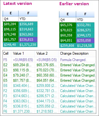
- The results appear in a two-pane grid, with the “Compare” file (typically older) on the left and the “To” file (typically newer) on the right.
- Details appear in a pane below the two grids.
- Changes are highlighted by color, indicating the type of change.
Understanding the Results:
- Worksheets are compared side-by-side. If there are multiple worksheets, you can navigate using the forward and back buttons on the horizontal scroll bar.
- Differences are highlighted with cell fill colors or text font colors, depending on the type of difference.
- The lower-left pane is a legend that shows what the colors mean.
Example:
If you have two versions of a sales report, Spreadsheet Compare can highlight changes in entered values (e.g., updated sales figures), calculated results (e.g., changes in totals), and formula corrections.
1.5 Third-Party Tools
In addition to Excel’s built-in features and Microsoft Spreadsheet Compare, several third-party tools are designed to compare Excel files. These tools often offer advanced features, such as detailed reporting, version control, and the ability to merge changes. Some popular options include:
- Araxis Merge: A professional tool for comparing and merging files, including Excel workbooks. It offers advanced features for identifying differences and resolving conflicts.
- Beyond Compare: A multi-platform utility for comparing files and folders. It supports Excel files and provides detailed reports of differences.
- XL Comparator: A specialized tool for comparing Excel files. It offers features such as side-by-side comparison, detailed reporting, and the ability to ignore specific differences.
These tools can be particularly useful for complex comparisons or when you need to track changes over time.
By using these methods, you can effectively compare data in two Excel workbooks and ensure data accuracy. Remember to visit COMPARE.EDU.VN for more detailed guides and tool comparisons to help you make the best choice for your specific needs.
2. What Are The Key Features To Look For In An Excel Comparison Tool?
When selecting an Excel comparison tool, it’s crucial to consider several key features to ensure that the tool meets your specific needs. These features can significantly impact the efficiency and accuracy of your data comparison process. Here are some of the most important features to look for:
2.1 Side-By-Side Comparison
A side-by-side comparison feature allows you to view two Excel workbooks simultaneously, making it easier to visually identify differences. This feature is particularly useful for comparing worksheets with similar layouts and data structures.
Benefits of Side-By-Side Comparison:
- Visual Clarity: Easier to spot differences at a glance.
- Improved Accuracy: Reduces the risk of overlooking discrepancies.
- Enhanced Efficiency: Speeds up the comparison process by allowing you to directly compare data points.
Example:
Imagine you have two versions of a budget spreadsheet. A side-by-side comparison feature would allow you to view both versions simultaneously, highlighting any changes in figures, formulas, or formatting.
2.2 Difference Highlighting
Difference highlighting automatically identifies and highlights discrepancies between two Excel workbooks. This feature is essential for quickly locating and addressing inconsistencies in your data.
Types of Difference Highlighting:
- Cell Value Differences: Highlights cells where the values have changed.
- Formula Differences: Identifies changes in formulas, including additions, deletions, or modifications.
- Formatting Differences: Highlights changes in cell formatting, such as font, color, and alignment.
- Structure Differences: Detects changes in the structure of the worksheet, such as added or deleted rows and columns.
Example:
Suppose you are comparing two versions of a sales report. Difference highlighting would automatically highlight any changes in sales figures, new or modified formulas, and alterations in formatting, allowing you to focus on the areas that need attention.
2.3 Detailed Reporting
A detailed reporting feature provides a comprehensive summary of the differences between two Excel workbooks. This report typically includes a list of all changes, along with details about the type of change, the location of the change, and the original and modified values.
Benefits of Detailed Reporting:
- Comprehensive Overview: Provides a complete summary of all changes.
- Improved Auditability: Creates a record of all modifications for auditing purposes.
- Enhanced Collaboration: Facilitates collaboration by providing a clear and concise summary of changes for team members.
Example:
A detailed report might list all the changes made to a financial statement, including specific cell values, formula modifications, and formatting alterations. This report can be used to verify the accuracy of the changes and ensure compliance with accounting standards.
2.4 Ignore Options
Ignore options allow you to exclude specific types of differences from the comparison. This feature is useful for focusing on the most relevant changes and filtering out noise.
Types of Ignore Options:
- Ignore Formatting: Excludes formatting differences from the comparison.
- Ignore Case: Ignores differences in capitalization.
- Ignore White Space: Ignores differences in white space (e.g., extra spaces or tabs).
- Ignore Comments: Excludes differences in comments from the comparison.
Example:
If you are comparing two versions of a document and you are only interested in content changes, you can use the ignore formatting option to exclude formatting differences from the comparison. This will allow you to focus on the actual changes in the text.
2.5 Version Control Integration
Version control integration allows you to connect your Excel comparison tool with a version control system, such as Git or SharePoint. This feature enables you to track changes over time, revert to previous versions, and collaborate more effectively with team members.
Benefits of Version Control Integration:
- Change Tracking: Keeps a record of all changes made to the workbook.
- Reversion: Allows you to revert to previous versions if necessary.
- Collaboration: Facilitates collaboration by providing a shared repository for Excel files.
Example:
If you are working on a project with multiple team members, version control integration would allow you to track all the changes made to the Excel workbook, revert to previous versions if necessary, and ensure that everyone is working on the latest version of the file.
2.6 Merge Capabilities
Merge capabilities allow you to combine changes from two Excel workbooks into a single workbook. This feature is useful for resolving conflicts and integrating updates from different sources.
Types of Merge Capabilities:
- Manual Merge: Allows you to selectively merge changes from one workbook to another.
- Automatic Merge: Automatically merges all changes from one workbook to another.
- Conflict Resolution: Provides tools for resolving conflicting changes.
Example:
Suppose you have two team members working on the same budget spreadsheet. Merge capabilities would allow you to combine their changes into a single workbook, resolving any conflicts that may arise.
2.7 User-Friendly Interface
A user-friendly interface is essential for ensuring that the Excel comparison tool is easy to use and understand. The interface should be intuitive and well-organized, with clear instructions and helpful tooltips.
Elements of a User-Friendly Interface:
- Intuitive Navigation: Easy to navigate and find the features you need.
- Clear Instructions: Provides clear and concise instructions.
- Helpful Tooltips: Offers helpful tooltips to guide you through the comparison process.
- Customizable Layout: Allows you to customize the layout to suit your preferences.
Example:
A user-friendly interface would provide clear instructions on how to select the Excel workbooks you want to compare, choose the comparison options, and interpret the results. It would also offer helpful tooltips to explain the different features and options.
2.8 Compatibility
Compatibility with different versions of Excel and operating systems is an important consideration when selecting an Excel comparison tool. The tool should be compatible with the versions of Excel and operating systems that you and your team members use.
Compatibility Considerations:
- Excel Versions: Ensure the tool is compatible with the versions of Excel you use (e.g., Excel 2010, Excel 2013, Excel 2016, Excel 2019, Excel 365).
- Operating Systems: Ensure the tool is compatible with the operating systems you use (e.g., Windows, macOS).
- File Formats: Ensure the tool supports the file formats you use (e.g., .xls, .xlsx, .xlsm).
Example:
If you and your team members use different versions of Excel, it is important to choose an Excel comparison tool that is compatible with all of those versions. This will ensure that everyone can use the tool effectively.
By considering these key features, you can select an Excel comparison tool that meets your specific needs and helps you efficiently and accurately compare data in two Excel workbooks. For more detailed reviews and comparisons of Excel comparison tools, visit COMPARE.EDU.VN.
3. How Can I Use Excel Formulas To Compare Two Columns Of Data?
Excel formulas provide a powerful way to compare two columns of data, allowing you to identify matches, differences, and other patterns. By using formulas like IF, EXACT, MATCH, and conditional formatting, you can efficiently analyze your data and extract valuable insights.
3.1 Using The IF Function For Basic Comparison
The IF function is a fundamental tool for comparing data in Excel. It allows you to perform a logical test and return different values based on whether the test is true or false.
How to Use the IF Function to Compare Two Columns:
- Open Your Excel Workbook: Open the Excel workbook containing the two columns you want to compare.
- Select a Cell for Comparison: In a new column, select the first cell where you want to display the comparison result.
- Enter the
IFFormula:- Use the
IFfunction to compare the values in the corresponding cells of the two columns. - The syntax for
IFis=IF(logical_test, value_if_true, value_if_false).logical_test: The comparison you want to perform (e.g.,A1=B1).value_if_true: The value to return if the comparison is true (e.g., “Match”).value_if_false: The value to return if the comparison is false (e.g., “Mismatch”).
- Use the
- Example Formula:
=IF(A1=B1,"Match","Mismatch")- This formula compares the value in cell A1 with the value in cell B1. If they are the same, it returns “Match”; otherwise, it returns “Mismatch”.
- Drag the Formula Down: Apply the formula to all relevant cells in the column by dragging the fill handle (the small square at the bottom-right corner of the cell) down.
- Review the Results: The cells in the new column will now display “Match” or “Mismatch” based on whether the values in the corresponding cells are the same.
Example:
Suppose you have two columns of customer names in columns A and B. You can use the IF function to quickly identify which names are present in both columns and which are not.
3.2 Using The EXACT Function For Case-Sensitive Comparison
The EXACT function is used to compare two text strings, taking into account the case of the characters. This function is useful when you need to ensure that the text strings are exactly the same, including capitalization.
How to Use the EXACT Function to Compare Two Columns:
- Open Your Excel Workbook: Open the Excel workbook containing the two columns you want to compare.
- Select a Cell for Comparison: In a new column, select the first cell where you want to display the comparison result.
- Enter the
EXACTFormula:- Use the
EXACTfunction to compare the values in the corresponding cells of the two columns. - The syntax for
EXACTis=EXACT(text1, text2).text1: The first text string to compare (e.g.,A1).text2: The second text string to compare (e.g.,B1).
- Use the
- Combine with The
IFFunction:- To display “Match” or “Mismatch”, combine the
EXACTfunction with theIFfunction. =IF(EXACT(A1,B1), "Match", "Mismatch")- This formula compares the text in cell A1 with the text in cell B1. If they are exactly the same (including case), it returns “Match”; otherwise, it returns “Mismatch”.
- To display “Match” or “Mismatch”, combine the
- Drag the Formula Down: Apply the formula to all relevant cells in the column by dragging the fill handle down.
- Review the Results: The cells in the new column will now display “Match” or “Mismatch” based on whether the text in the corresponding cells is exactly the same.
Example:
Suppose you have two columns of product codes in columns A and B. The EXACT function can help you ensure that the product codes are identical, including the case of the letters.
3.3 Using The MATCH Function To Find Matching Values
The MATCH function searches for a specified item in a range of cells and returns the relative position of that item in the range. This function is useful for determining whether a value in one column exists in another column.
How to Use the MATCH Function to Compare Two Columns:
- Open Your Excel Workbook: Open the Excel workbook containing the two columns you want to compare.
- Select a Cell for Comparison: In a new column, select the first cell where you want to display the comparison result.
- Enter the
MATCHFormula:- Use the
MATCHfunction to search for values in one column within another column. - The syntax for
MATCHis=MATCH(lookup_value, lookup_array, [match_type]).lookup_value: The value you want to search for (e.g.,A1).lookup_array: The range of cells where you want to search for the value (e.g.,B:Bfor the entire column B).[match_type]: Specify0for an exact match.
- Use the
- Combine with The
ISNUMBERFunction:- To display “Match” or “Mismatch”, combine the
MATCHfunction with theISNUMBERfunction. =IF(ISNUMBER(MATCH(A1,B:B,0)), "Match", "Mismatch")- This formula searches for the value in cell A1 within column B. If a match is found,
MATCHreturns the position of the match, andISNUMBERreturnsTRUE. If no match is found,MATCHreturns an error, andISNUMBERreturnsFALSE.
- To display “Match” or “Mismatch”, combine the
- Drag the Formula Down: Apply the formula to all relevant cells in the column by dragging the fill handle down.
- Review the Results: The cells in the new column will now display “Match” or “Mismatch” based on whether the values in column A exist in column B.
Example:
Suppose you have a list of email addresses in column A and a list of registered users in column B. The MATCH function can help you identify which email addresses in column A are also registered users in column B.
3.4 Using Conditional Formatting To Highlight Differences
Conditional formatting can be combined with formulas to highlight differences between two columns visually. This method is useful for quickly identifying discrepancies and patterns in your data.
How to Use Conditional Formatting to Highlight Differences:
- Open Your Excel Workbook: Open the Excel workbook containing the two columns you want to compare.
- Select the Data Range: Select the range of cells you want to format (e.g., column A).
- Go to Conditional Formatting:
- Click on the “Home” tab.
- In the “Styles” group, click “Conditional Formatting.”
- Choose “New Rule.”
- Create a New Rule:
- Select “Use a formula to determine which cells to format.”
- Enter a formula that compares the cell in the selected range to the corresponding cell in the other column. For example, to highlight cells in column A that do not match the corresponding cells in column B, the formula would be
=A1<>B1. - Click “Format” to choose how you want the differences to be highlighted (e.g., fill color, font color).
- Click “OK” to apply the formatting.
- Apply to All Cells: Ensure that the conditional formatting rule applies to all the cells in your selected range.
- Review the Results: Any cells in column A that are different from their counterparts in column B will now be highlighted according to the formatting you chose.
Example:
Suppose you have two columns of sales figures in columns A and B. Using conditional formatting, you can highlight any cells in column A that have different values than their corresponding cells in column B, making it easy to identify discrepancies in your sales data.
By using these Excel formulas and techniques, you can efficiently compare two columns of data and extract valuable insights. For more advanced tips and tricks, visit COMPARE.EDU.VN.
4. What Is The Best Way To Synchronize Data Between Two Excel Sheets?
Synchronizing data between two Excel sheets ensures that changes made in one sheet are automatically reflected in the other, maintaining consistency and accuracy. Several methods can achieve this, including using formulas, Power Query, and VBA.
4.1 Using Formulas To Link Cells
Formulas are a simple way to link individual cells between two Excel sheets, ensuring that changes in one cell are automatically reflected in the other.
How to Use Formulas to Link Cells:
- Open Your Excel Workbook: Open the Excel workbook containing the two sheets you want to synchronize.
- Select the Destination Cell: In the destination sheet, select the cell where you want to display the value from the source sheet.
- Enter the Formula:
- Type
=followed by the sheet name, an exclamation mark (!), and the cell reference from the source sheet. - For example, if you want to link cell A1 from Sheet1 to cell B1 in Sheet2, the formula in Sheet2, cell B1, would be
=Sheet1!A1.
- Type
- Press Enter: Press Enter to apply the formula. The value from the source cell will now appear in the destination cell.
- Repeat for Other Cells: Repeat this process for all the cells you want to synchronize between the two sheets.
Example:
If you have a master sheet with a list of product names and prices, you can use formulas to link these values to other sheets, such as sales reports or inventory lists. Any changes made to the product names or prices in the master sheet will automatically be reflected in the other sheets.
4.2 Using Power Query To Create A Dynamic Link
Power Query is a powerful data transformation and integration tool built into Excel. It allows you to create a dynamic link between two Excel sheets, ensuring that changes in the source sheet are automatically updated in the destination sheet.
How to Use Power Query to Create a Dynamic Link:
- Open Your Excel Workbook: Open the Excel workbook containing the two sheets you want to synchronize.
- Convert Data to Tables: Convert the data in both sheets to Excel tables. To do this, select the data range in each sheet and press
Ctrl+T. Ensure that the “My table has headers” checkbox is selected if your data includes headers. - Import Data into Power Query:
- Go to the “Data” tab and click “From Table/Range.” This will open the Power Query Editor.
- In the Power Query Editor, make any necessary transformations to the data, such as filtering, sorting, or renaming columns.
- Click “Close & Load” to load the data back into an Excel sheet.
- Create a Connection Only:
- Instead of loading the data directly into a sheet, you can create a connection only. In the “Close & Load” dropdown, select “Close & Load To…”
- Choose “Only Create Connection” and click “Load.”
- Create a New Query to Link the Data:
- Go to the “Data” tab and click “Get Data” > “Combine Queries” > “Merge.”
- In the Merge dialog box, select the first table and then select the second table.
- Choose the columns to match between the two tables and select the join type (e.g., “Left Outer” to include all rows from the first table and matching rows from the second table).
- Click “OK” to create the merged query.
- Expand the Merged Columns:
- In the Power Query Editor, click the expand button (two arrows pointing in opposite directions) in the header of the merged column.
- Select the columns you want to include from the second table and click “OK.”
- Load the Data:
- Click “Close & Load” to load the synchronized data into a new Excel sheet.
- Refresh the Data:
- To update the data, go to the “Data” tab and click “Refresh All.” This will update the data in the destination sheet with any changes made in the source sheet.
Example:
Suppose you have two sheets with customer data. Sheet1 contains customer names and contact information, and Sheet2 contains customer purchase history. Using Power Query, you can merge these two sheets based on a common identifier, such as customer ID, to create a synchronized view of customer data.
4.3 Using VBA To Automate Data Synchronization
VBA (Visual Basic for Applications) allows you to automate data synchronization between two Excel sheets using custom code. This method is useful for more complex synchronization scenarios where you need to perform custom logic or handle specific events.
How to Use VBA to Automate Data Synchronization:
- Open Your Excel Workbook: Open the Excel workbook containing the two sheets you want to synchronize.
- Open the VBA Editor: Press
Alt+F11to open the VBA Editor. - Insert a New Module: In the VBA Editor, go to “Insert” > “Module” to insert a new module.
- Write the VBA Code:
- Write VBA code to synchronize the data between the two sheets. Here is an example code:
Private Sub Worksheet_Change(ByVal Target As Range)
    Dim SourceSheet As Worksheet
    Dim DestSheet As Worksheet
    Dim KeyCells As Range

    Set SourceSheet = ThisWorkbook.Sheets("Sheet1") ' Change "Sheet1" to your source sheet name
    Set DestSheet = ThisWorkbook.Sheets("Sheet2")   ' Change "Sheet2" to your destination sheet name

    ' Specify the range of cells you want to monitor for changes
    Set KeyCells = SourceSheet.Range("A1:Z100")

    If Not Application.Intersect(KeyCells, Target) Is Nothing Then
        ' Disable events to prevent recursive triggering
        Application.EnableEvents = False

        ' Loop through each changed cell in the target range
        For Each cell In Target
            ' Find the corresponding cell in the destination sheet
            Dim SourceRow As Long, SourceCol As Long
            SourceRow = cell.Row
            SourceCol = cell.Column

            DestSheet.Cells(SourceRow, SourceCol).Value = cell.Value
        Next cell

        ' Re-enable events
        Application.EnableEvents = True
    End If
End Sub-
Explanation of the Code:
Private Sub Worksheet_Change(ByVal Target As Range): This is an event handler that triggers whenever a change is made to a worksheet.Dim SourceSheet As Worksheet,Dim DestSheet As Worksheet,Dim KeyCells As Range: These lines declare variables to hold references to the source sheet, destination sheet, and the range of cells to monitor for changes.Set SourceSheet = ThisWorkbook.Sheets("Sheet1"): Sets the source sheet to “Sheet1”. Change"Sheet1"to the name of your source sheet.Set DestSheet = ThisWorkbook.Sheets("Sheet2"): Sets the destination sheet to “Sheet2”. Change"Sheet2"to the name of your destination sheet.Set KeyCells = SourceSheet.Range("A1:Z100"): Sets the range of cells in the source sheet that will trigger the synchronization. Change"A1:Z100"to the range you want to monitor.If Not Application.Intersect(KeyCells, Target) Is Nothing Then: Checks if the changed cell is within the specified range (KeyCells).Application.EnableEvents = False: Disables events to prevent the code from triggering itself in a loop.- The
For Each cell In Targetloop iterates through each cell that was changed. DestSheet.Cells(SourceRow, SourceCol).Value = cell.Value: Copies the value from the changed cell in the source sheet to the corresponding cell in the destination sheet.Application.EnableEvents = True: Re-enables events after the synchronization is complete.
-
Insert the Code into the Source Sheet:
- In the VBA Editor, double-click on the source sheet in the “Project” window (e.g., “Sheet1 (Sheet1)”).
- Paste the VBA code into the code window for the source sheet.
-
Customize the Code:
- Modify the code to suit your specific needs. For example, you can change the sheet names, the range of cells to monitor, and the synchronization logic.
-
Save the Workbook:
- Save the Excel workbook as a macro-enabled workbook (
.xlsm).
- Save the Excel workbook as a macro-enabled workbook (
-
Test the Code:
- Make changes to the cells in the specified range in the source sheet. The changes should automatically be reflected in the destination sheet.
-
Enable Macros:
- If prompted, enable macros when you open the workbook.
Example:
Suppose you have a master sheet with a list of product names and prices. You can use VBA code to automatically update the prices in other sheets whenever the prices are changed in the master sheet. This ensures that all sheets are always synchronized with the latest price information.
By using these methods, you can effectively synchronize data between two Excel sheets and ensure data consistency. For more detailed tutorials and examples, visit compare.edu.vn.
5. How Do I Compare Data In Two Excel Workbooks For Duplicates?
Identifying duplicate data in two Excel workbooks is