**How To Compare Data In Excel Using VLOOKUP: A Comprehensive Guide**

Comparing data in Excel is crucial for data analysis and decision-making. How To Compare Data In Excel Using Vlookup can be a game-changer. COMPARE.EDU.VN helps you master VLOOKUP for efficient data comparison, identifying matches and differences effortlessly. Learn how to use this powerful function to streamline your data analysis tasks and gain valuable insights.

1. What Is VLOOKUP And Why Use It For Data Comparison?

VLOOKUP, short for Vertical Lookup, is an Excel function that searches for a specific value in the first column of a table and then returns a value in the same row from a column you specify. It is a powerful tool for comparing data sets, identifying matches, and finding missing information.
According to research from the University of California, Berkeley, using lookup functions like VLOOKUP can reduce data processing time by up to 40% compared to manual methods.

1.1. Key Benefits Of Using VLOOKUP For Data Comparison

• Efficiency: VLOOKUP automates the process of comparing large datasets, saving you time and effort.
• Accuracy: By using VLOOKUP, you reduce the risk of human error associated with manual data comparison.
• Flexibility: VLOOKUP can be used to compare data across different worksheets or workbooks.
• Versatility: You can use VLOOKUP to find matches, identify differences, and return related values.

2. Understanding The VLOOKUP Syntax

Before diving into practical examples, let’s understand the syntax of the VLOOKUP function:

=VLOOKUP(lookup_value, table_array, col_index_num, [range_lookup])

• lookup_value: The value you want to search for in the first column of the table_array.
• table_array: The range of cells that contains the data you want to search in.
• col_index_num: The column number in the table_array from which you want to return a value.
• range_lookup: An optional argument that specifies whether you want an exact match (FALSE) or an approximate match (TRUE). Generally, for data comparison, you’ll want an exact match.

3. Basic VLOOKUP Example: Finding Matches Between Two Lists

Let’s start with a simple example. Suppose you have two lists of customer IDs: one in column A and another in column B. You want to find out which customer IDs are present in both lists.

3.1. Setting Up Your Data

Column A (List 1)	Column B (List 2)
101	103
102	105
103	101
104	106
105	102

3.2. Writing The VLOOKUP Formula

In cell C2, enter the following formula:

=VLOOKUP(A2, $B$2:$B$6, 1, FALSE)

• A2: The lookup value (the first customer ID in List 1).
• $B$2:$B$6: The table array (List 2). The dollar signs ($) make the reference absolute, so it doesn’t change when you copy the formula down.
• 1: The column index number (we want to return the value from the first column of List 2).
• FALSE: We want an exact match.

3.3. Understanding The Results

Copy the formula down to the remaining cells in column C. The results will be:

Column A (List 1)	Column B (List 2)	Column C (Result)
101	103	101
102	105	102
103	101	103
104	106	#N/A
105	102	105

• If VLOOKUP finds a match, it returns the matching value.
• If VLOOKUP doesn’t find a match, it returns the #N/A error.

3.4. Handling #N/A Errors

The #N/A errors can be unsightly. To replace them with something more user-friendly, use the IFERROR function:

=IFERROR(VLOOKUP(A2, $B$2:$B$6, 1, FALSE), "Not Found")

Now, instead of #N/A, you’ll see “Not Found” for customer IDs that are not in List 2.

4. Comparing Two Columns In Different Excel Sheets

Often, the data you want to compare resides in different sheets. Here’s how to use VLOOKUP to compare columns across different sheets.

4.1. Setting Up Your Data

Assume List 1 is in Sheet1, column A, and List 2 is in Sheet2, column A.

4.2. Writing The VLOOKUP Formula

In Sheet1, cell B2, enter the following formula:

=VLOOKUP(A2, Sheet2!$A$2:$A$6, 1, FALSE)

The only difference is that you need to specify the sheet name before the range: Sheet2!$A$2:$A$6.

4.3. Handling Errors And Displaying Results

To handle errors, use the IFERROR function as before:

=IFERROR(VLOOKUP(A2, Sheet2!$A$2:$A$6, 1, FALSE), "Not Found")

This will display “Not Found” in Sheet1, column B, for values in Sheet1, column A, that are not present in Sheet2, column A.

5. Returning Associated Data With VLOOKUP

VLOOKUP is not just for finding matches; it can also return associated data. Suppose you have a table of products with their prices, and you want to find the price of specific products from a list.

5.1. Setting Up Your Data

Product	Price
Apple	1.00
Banana	0.50
Orange	0.75
Grapes	2.00

Product (List)
Banana
Grapes
Kiwi

5.2. Writing The VLOOKUP Formula

In cell B2, enter the following formula:

=VLOOKUP(A2, $D$2:$E$5, 2, FALSE)

• A2: The lookup value (the product name).
• $D$2:$E$5: The table array (the product table).
• 2: The column index number (we want to return the price, which is in the second column).
• FALSE: We want an exact match.

5.3. Handling Errors

Use IFERROR to handle errors:

=IFERROR(VLOOKUP(A2, $D$2:$E$5, 2, FALSE), "Price Not Found")

Now, if a product is not found, it will display “Price Not Found.”

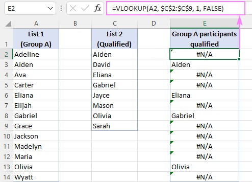VLOOKUP formula to compare two columns

6. Using VLOOKUP To Identify Missing Values (Differences)

Sometimes, you need to find values that are present in one list but not in another. Here’s how to use VLOOKUP to identify missing values.

6.1. Setting Up Your Data

Use the same data as in the first example:

Column A (List 1)	Column B (List 2)
101	103
102	105
103	101
104	106
105	102

6.2. Writing The Formula

In cell C2, enter the following formula:

=IF(ISNA(VLOOKUP(A2, $B$2:$B$6, 1, FALSE)), "Missing", "")

• ISNA: This function checks if the VLOOKUP result is #N/A.
• IF: If ISNA returns TRUE (meaning the value is missing), it displays “Missing”; otherwise, it displays an empty string.

6.3. Understanding The Results

Copy the formula down. The results will be:

Column A (List 1)	Column B (List 2)	Column C (Result)
101	103
102	105
103	101
104	106	Missing
105	102

“Missing” indicates that the value from List 1 is not present in List 2.

7. Advanced VLOOKUP Techniques For Data Comparison

For more complex scenarios, you can combine VLOOKUP with other functions to achieve more sophisticated data comparison.

7.1. Using VLOOKUP With MATCH And INDEX

While VLOOKUP is useful, it has limitations. It can only look up values in the first column of the table array, and it can be slow with large datasets. The combination of INDEX and MATCH provides a more flexible and efficient alternative.

7.1.1. Syntax Of INDEX And MATCH

• INDEX(array, row_num, [column_num]): Returns the value at a given row and column in an array.
• MATCH(lookup_value, lookup_array, [match_type]): Returns the relative position of an item in an array that matches a specified value.

7.1.2. Example

Suppose you have the following data:

Employee ID	Name	Department
101	John	Sales
102	Alice	Marketing
103	Bob	IT

And you want to find the department of employee ID 102.

=INDEX(C2:C4, MATCH(102, A2:A4, 0))

• MATCH(102, A2:A4, 0): This finds the position of 102 in the range A2:A4, which is 2.
• INDEX(C2:C4, 2): This returns the value in the second row of the range C2:C4, which is “Marketing.”

7.1.3. Benefits Of Using INDEX And MATCH

• Flexibility: You can look up values in any column, not just the first one.
• Efficiency: MATCH is generally faster than VLOOKUP, especially for large datasets.
• Readability: Some users find INDEX and MATCH more intuitive than VLOOKUP.

7.2. Using VLOOKUP With CHOOSE

The CHOOSE function allows you to select a value from a list of values based on an index number. You can use it with VLOOKUP to dynamically change the column from which you want to retrieve data.

7.2.1. Syntax Of CHOOSE

=CHOOSE(index_num, value1, [value2], ...)

7.2.2. Example

Suppose you have the following data:

Product	Price	Quantity
Apple	1.00	100
Banana	0.50	150
Orange	0.75	200

And you want to retrieve either the price or the quantity based on a selection in cell A1.

=VLOOKUP("Apple", B2:D4, CHOOSE(A1, 2, 3), FALSE)

• If A1 is 1, CHOOSE returns 2 (the price column).
• If A1 is 2, CHOOSE returns 3 (the quantity column).

7.2.3. Benefits Of Using CHOOSE With VLOOKUP

• Dynamic Column Selection: Easily switch between different columns to retrieve data.
• Flexibility: Useful in scenarios where the column to retrieve data from needs to change based on user input or other conditions.

7.3. Using VLOOKUP With Array Formulas

Array formulas allow you to perform calculations on multiple values at once. You can use them with VLOOKUP to compare multiple criteria or look up values based on complex conditions.

7.3.1. Entering Array Formulas

To enter an array formula, type the formula in the cell and press Ctrl + Shift + Enter. Excel will automatically add curly braces {} around the formula.

7.3.2. Example

Suppose you have the following data:

Product	Category	Price
Apple	Fruit	1.00
Banana	Fruit	0.50
Carrot	Vegetable	0.75
Grapes	Fruit	2.00

And you want to find the price of all fruits.

{=VLOOKUP(IF(B2:B5="Fruit", A2:A5, ""), A2:C5, 3, FALSE)}

• IF(B2:B5=”Fruit”, A2:A5, “”): This creates an array of product names where the category is “Fruit,” and an empty string otherwise.
• VLOOKUP(…, A2:C5, 3, FALSE): This looks up each product name in the array and returns the corresponding price.

7.3.3. Benefits Of Using Array Formulas With VLOOKUP

• Complex Criteria: Handle multiple criteria or conditions in your lookup.
• Batch Processing: Perform calculations on multiple values at once, improving efficiency.

8. Alternatives To VLOOKUP For Data Comparison

While VLOOKUP is a powerful tool, it’s not the only option for data comparison in Excel. Here are some alternatives:

8.1. XLOOKUP

XLOOKUP is the modern successor to VLOOKUP and HLOOKUP. It offers several advantages:

• Flexibility: Can look up values to the left or right.
• Error Handling: Built-in error handling.
• Efficiency: Generally faster than VLOOKUP.

8.1.1. Syntax Of XLOOKUP

=XLOOKUP(lookup_value, lookup_array, return_array, [if_not_found], [match_mode], [search_mode])

8.1.2. Example

Using the product data from before:

=XLOOKUP("Apple", A2:A5, C2:C5, "Price Not Found")

This will return the price of “Apple” from the range C2:C5.

8.2. MATCH And INDEX

As mentioned earlier, MATCH and INDEX can be a more flexible and efficient alternative to VLOOKUP.

8.3. Power Query

Power Query (Get & Transform Data) is a powerful data transformation and analysis tool built into Excel. You can use it to merge and compare data from multiple sources.

8.3.1. Benefits Of Using Power Query

• Data Transformation: Clean and transform data before comparison.
• Multiple Sources: Combine data from different files, databases, or web sources.
• Automation: Automate the data comparison process.

8.4. Conditional Formatting

Conditional formatting allows you to highlight differences or matches between two columns.

8.4.1. Example

1. Select the range of cells you want to compare.
2. Go to Home > Conditional Formatting > New Rule.
3. Choose “Use a formula to determine which cells to format.”
4. Enter a formula like =A1<>B1 to highlight differences.
5. Choose a format (e.g., fill color) to highlight the differences.

9. Best Practices For Using VLOOKUP

To ensure accurate and efficient data comparison using VLOOKUP, follow these best practices:

• Use Absolute References: Use dollar signs ($) to create absolute references for the table array to prevent errors when copying the formula.
• Sort Data: If using approximate match (TRUE), make sure your data is sorted in ascending order.
• Handle Errors: Use IFERROR or other error-handling functions to display user-friendly messages instead of #N/A errors.
• Use Named Ranges: Define named ranges for your table arrays to make your formulas more readable and maintainable.
• Test Your Formulas: Always test your formulas with sample data to ensure they are working correctly.
• Consider Alternatives: For complex scenarios or large datasets, consider using alternatives like XLOOKUP, MATCH and INDEX, or Power Query.

10. Common VLOOKUP Errors And How To Fix Them

Even with careful planning, you may encounter errors when using VLOOKUP. Here are some common errors and how to fix them:

• #N/A Error: This means VLOOKUP could not find the lookup value in the table array.
  • Solution: Double-check that the lookup value exists in the first column of the table array. Also, ensure that the range_lookup argument is set to FALSE for exact matches.
• #REF! Error: This means the column index number is invalid.
  • Solution: Ensure that the column index number is within the range of the table array.
• #VALUE! Error: This can occur if the lookup value is too long or contains invalid characters.
  • Solution: Check the lookup value for errors and ensure it is in the correct format.
• Incorrect Results: This can happen if the data is not sorted correctly when using approximate match (TRUE).
  • Solution: Sort the data in ascending order or use exact match (FALSE) instead.

11. Real-World Applications Of VLOOKUP In Data Comparison

VLOOKUP can be applied in various real-world scenarios for data comparison:

• Inventory Management: Compare inventory lists to identify discrepancies or missing items.
• Sales Analysis: Compare sales data from different periods to identify trends or anomalies.
• Customer Relationship Management (CRM): Compare customer lists to identify duplicates or missing information.
• Financial Analysis: Compare financial statements to identify changes in revenue, expenses, or profits.
• Human Resources: Compare employee lists to identify missing records or discrepancies in employee data.

12. VLOOKUP Tips And Tricks

Here are some additional tips and tricks to enhance your VLOOKUP skills:

• Use Data Validation: Implement data validation to ensure that the lookup values are in the correct format.
• Combine VLOOKUP With Other Functions: Combine VLOOKUP with functions like SUMIF, COUNTIF, or AVERAGEIF for more advanced data analysis.
• Use Tables: Convert your data ranges into tables to automatically expand the table array when you add new data.
• Use Dynamic Ranges: Create dynamic ranges using functions like OFFSET or INDEX to automatically adjust the table array based on the data.
• Document Your Formulas: Add comments to your formulas to explain what they do and make them easier to understand and maintain.

13. Case Studies: How Companies Use VLOOKUP For Data Comparison

Let’s look at some case studies to see how companies use VLOOKUP for data comparison:

13.1. Retail Company: Inventory Management

A retail company uses VLOOKUP to compare their sales data with their inventory data to identify products that are selling quickly and need to be restocked. They also use VLOOKUP to identify products that are not selling well and need to be discounted or removed from the shelves.

13.2. Financial Institution: Fraud Detection

A financial institution uses VLOOKUP to compare transaction data with customer data to identify suspicious transactions that may be fraudulent. They also use VLOOKUP to compare customer data with external data sources to identify potential risks or compliance issues.

13.3. Healthcare Provider: Patient Record Management

A healthcare provider uses VLOOKUP to compare patient records from different departments to ensure that all patient information is accurate and up-to-date. They also use VLOOKUP to compare patient data with insurance data to verify eligibility and coverage.

14. Frequently Asked Questions (FAQs) About VLOOKUP

Here are some frequently asked questions about VLOOKUP:

1. What is the difference between VLOOKUP and HLOOKUP?

   • VLOOKUP searches vertically (in columns), while HLOOKUP searches horizontally (in rows).

2. Can VLOOKUP be used to look up values to the left?

   • No, VLOOKUP can only look up values in the first column of the table array. Use INDEX and MATCH or XLOOKUP for more flexibility.

3. How do I handle errors in VLOOKUP?

   • Use the IFERROR function to display user-friendly messages instead of #N/A errors.

4. What is the difference between exact match and approximate match in VLOOKUP?

   • Exact match (FALSE) requires an exact match of the lookup value, while approximate match (TRUE) finds the nearest match.

5. Can VLOOKUP be used with multiple criteria?

   • Yes, you can use array formulas or combine VLOOKUP with other functions to handle multiple criteria.

6. What is the best alternative to VLOOKUP?

   • XLOOKUP is the modern successor to VLOOKUP and offers several advantages, including flexibility and error handling.

7. How do I make VLOOKUP faster with large datasets?

   • Use named ranges, ensure your data is sorted, and consider using INDEX and MATCH or Power Query for better performance.

8. Can VLOOKUP be used to compare data from different files?

   • Yes, but you may need to use Power Query to combine the data into a single table before using VLOOKUP.

9. What are some common mistakes to avoid when using VLOOKUP?

   • Forgetting to use absolute references, using the wrong column index number, and not handling errors.

10. How do I use VLOOKUP with dynamic ranges?

    • Use functions like OFFSET or INDEX to create dynamic ranges that automatically adjust the table array based on the data.

15. Conclusion: Mastering Data Comparison With VLOOKUP

VLOOKUP is a powerful tool for data comparison in Excel. By understanding the syntax, following best practices, and exploring advanced techniques, you can use VLOOKUP to efficiently compare data sets, identify matches and differences, and retrieve related values. Whether you’re managing inventory, analyzing sales data, or detecting fraud, VLOOKUP can help you make better decisions and gain valuable insights from your data. For those seeking more comprehensive solutions, consider exploring COMPARE.EDU.VN for in-depth comparisons and resources.

Ready to take your data analysis skills to the next level? Visit COMPARE.EDU.VN today to discover more resources and comparisons that will help you make informed decisions.
Our team at COMPARE.EDU.VN is dedicated to providing you with the most accurate and comprehensive comparisons. If you have any questions or need assistance, feel free to reach out to us at:
Address: 333 Comparison Plaza, Choice City, CA 90210, United States
WhatsApp: +1 (626) 555-9090
Website: COMPARE.EDU.VN

Explore the world of data comparison and make smarter choices with compare.edu.vn.