Are you struggling with How To Compare Data In Excel And Highlight Differences? Don’t worry! COMPARE.EDU.VN provides a comprehensive guide to effectively compare data in Excel, identify disparities, and emphasize key insights. This article offers various methods, from simple formulas to advanced techniques, helping you analyze data and pinpoint discrepancies. Discover how to use Excel to compare datasets efficiently, highlighting both matches and differences.
1. Understanding the Need to Compare Data in Excel
Data comparison is a fundamental task in various fields, from finance and accounting to sales and marketing. Excel, with its robust features, offers numerous ways to perform this task. However, knowing how to compare data in Excel and highlight differences effectively is crucial for accurate analysis and decision-making.
1.1. Why Compare Data in Excel?
Comparing data in Excel allows you to:
- Identify discrepancies and errors
- Track changes over time
- Validate data accuracy
- Find duplicate entries
- Analyze trends and patterns
1.2. Who Benefits from Comparing Data in Excel?
- Students (18-24): Comparing grades, research data, or course information.
- Consumers (24-55): Comparing product features, prices, or reviews before making a purchase.
- Professionals (24-65+): Comparing performance metrics, financial data, or project timelines.
2. Basic Techniques: Comparing Data Row by Row
The most straightforward method to compare data in Excel involves comparing data row by row. This can be achieved using simple formulas and functions.
2.1. Using the IF Function
The IF function is a fundamental tool for comparing data in Excel. It allows you to specify a condition and return different values based on whether the condition is true or false.
2.1.1. Formula for Matches
To find cells within the same row having the same content, use the following formula:
=IF(A2=B2,"Match","")
This formula compares the values in cells A2 and B2. If they are equal, it returns “Match”; otherwise, it returns an empty string.
2.1.2. Formula for Differences
To find cells in the same row with different values, use the following formula:
=IF(A2<>B2,"No match","")
This formula compares the values in cells A2 and B2. If they are different, it returns “No match”; otherwise, it returns an empty string.
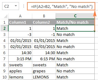
2.1.3. Matches and Differences
You can combine both matches and differences in a single formula:
=IF(A2=B2,"Match","No match")
or
=IF(A2<>B2,"No match","Match")
2.2. Case-Sensitive Comparison with EXACT
The IF function ignores case when comparing text values. For a case-sensitive comparison, use the EXACT function.
2.2.1. Formula for Case-Sensitive Matches
=IF(EXACT(A2, B2), "Match", "")
This formula returns “Match” only if the values in cells A2 and B2 are identical, including the case.
2.2.2. Formula for Case-Sensitive Differences
=IF(EXACT(A2, B2), "Match", "Unique")
This formula returns “Match” if the values are identical, and “Unique” if they are different.
3. Comparing Multiple Columns for Matches
When dealing with multiple columns, you may need to compare data across several columns to find matches or unique values.
3.1. Finding Matches in All Cells Within the Same Row
To find rows with the same values in all cells, use an IF formula with an AND statement.
3.1.1. Using the AND Function
=IF(AND(A2=B2, A2=C2), "Full match", "")
This formula checks if the values in cells A2, B2, and C2 are all equal. If they are, it returns “Full match”; otherwise, it returns an empty string.
3.1.2. Using the COUNTIF Function
For tables with many columns, a more efficient solution is using the COUNTIF function.
=IF(COUNTIF($A2:$E2, $A2)=5, "Full match", "")
Here, 5 is the number of columns you are comparing. The formula counts how many cells in the range A2:E2 have the same value as A2. If the count equals the number of columns, it returns “Full match”.
3.2. Finding Matches in Any Two Cells in the Same Row
To compare columns for any two or more cells with the same values within the same row, use an IF formula with an OR statement.
3.2.1. Using the OR Function
=IF(OR(A2=B2, B2=C2, A2=C2), "Match", "")
This formula checks if any two cells among A2, B2, and C2 have the same value. If at least two cells match, it returns “Match”; otherwise, it returns an empty string.
3.2.2. Combining COUNTIF Functions
If you have many columns to compare, adding up several COUNTIF functions can be more efficient.
=IF(COUNTIF(B2:D2,A2)+COUNTIF(C2:D2,B2)+(C2=D2)=0,"Unique","Match")
This formula checks for matches between any two cells in the range and returns “Match” if any match is found; otherwise, it returns “Unique”.
4. Comparing Two Columns for Matches and Differences
When you have two lists of data and want to find values that are in one column but not in the other, you can use a combination of IF and COUNTIF functions.
4.1. Finding Values in Column A Not in Column B
The following formula searches across the entire column B for the value in cell A2. If no match is found, the formula returns “No match in B”; otherwise, it returns an empty string.
=IF(COUNTIF($B:$B, $A2)=0, "No match in B", "")
4.2. Alternative Formulas
You can also achieve the same result using an IF formula with the embedded ISERROR and MATCH functions:
=IF(ISERROR(MATCH($A2,$B$2:$B$10,0)),"No match in B","")
Or, by using the following array formula (remember to press Ctrl + Shift + Enter to enter it correctly):
=IF(SUM(--($B$2:$B$10=$A2))=0, " No match in B", "")
4.3. Identifying Matches and Differences
To identify both matches and differences, put some text for matches in the empty double quotes (“”) in any of the above formulas. For example:
=IF(COUNTIF($B:$B, $A2)=0, "No match in B", "Match in B")
5. Pulling Matches from Two Lists
Sometimes, you may need to pull matching entries from one list to another. Excel provides functions like VLOOKUP, INDEX MATCH, and XLOOKUP for this purpose.
5.1. Using the VLOOKUP Function
The VLOOKUP function searches for a value in the first column of a range and returns a value from a specified column in the same row.
=VLOOKUP(D2, $A$2:$B$6, 2, FALSE)
This formula compares the product names in column D against the names in column A and pulls a corresponding sales figure from column B if a match is found.
5.2. Using the INDEX MATCH Combination
The INDEX MATCH combination is a more powerful and versatile alternative to VLOOKUP.
=INDEX($B$2:$B$6, MATCH($D2, $A$2:$A$6, 0))
This formula achieves the same result as VLOOKUP but is more flexible and less prone to errors.
5.3. Using the XLOOKUP Function
The XLOOKUP function, available in Excel 2021 and Excel 365, is a modern replacement for VLOOKUP and INDEX MATCH.
=XLOOKUP(D2, $A$2:$A$6, $B$2:$B$6)
This formula simplifies the process of looking up values and is more intuitive than its predecessors.
6. Highlighting Matches and Differences
Excel’s Conditional Formatting feature allows you to visually highlight matches and differences between columns, making it easier to identify and analyze discrepancies.
6.1. Highlighting Matches and Differences in Each Row
To highlight data in Excel and highlight differences in column A that have identical entries in column B in the same row, follow these steps:
- Select the cells you want to highlight.
- Click Conditional formatting > New Rule… > Use a formula to determine which cells to format.
- Create a rule with the formula
=$B2=$A2(assuming that row 2 is the first row with data).
To highlight differences between column A and B, create a rule with this formula:
=$B2<>$A2
6.2. Highlighting Unique Entries in Each List
To highlight unique entries in each list, create conditional formatting rules with the following formulas:
- Highlight unique values in List 1 (column A):
=COUNTIF($C$2:$C$5, $A2)=0
- Highlight unique values in List 2 (column C):
=COUNTIF($A$2:$A$6, $C2)=0
6.3. Highlighting Matches (Duplicates) Between Two Columns
To highlight matches between two columns, adjust the COUNTIF formulas to find matches rather than differences:
- Highlight matches in List 1 (column A):
=COUNTIF($C$2:$C$5, $A2)>0
- Highlight matches in List 2 (column C):
=COUNTIF($A$2:$A$6, $C2)>0
7. Highlighting Row Differences and Matches in Multiple Columns
When comparing values in several columns row-by-row, you can use conditional formatting to highlight matches and the “Go To Special” feature to highlight differences.
7.1. Highlighting Row Matches
To highlight rows that have identical values in all columns, create a conditional formatting rule based on one of the following formulas:
=AND($A2=$B2, $A2=$C2)
or
=COUNTIF($A2:$C2, $A2)=3
Where A2, B2, and C2 are the top-most cells, and 3 is the number of columns to compare.
7.2. Highlighting Row Differences
To quickly highlight cells with different values in each individual row, use Excel’s “Go To Special” feature:
- Select the range of cells you want to compare.
- On the Home tab, go to Editing group, and click Find & Select > Go To Special…
- Select Row differences and click the OK button.
- The cells whose values are different from the comparison cell in each row are colored.
8. Comparing Two Cells in Excel
Comparing two cells is a specific case of comparing two columns row-by-row.
8.1. Formulas for Comparison
To compare cells A1 and C1, use the following formulas:
- For matches:
=IF(A1=C1, "Match", "")
- For differences:
=IF(A1<>C1, "Difference", "")
9. Formula-Free Way to Compare Two Columns/Lists
For a formula-free solution, consider using add-ins like “Compare Two Tables” in Ablebits Ultimate Suite. This tool simplifies the process of comparing lists and highlighting matches and differences.
9.1. Using the Compare Tables Add-In
- Start by clicking the Compare Tables button on the Ablebits Data tab.
- Select the first and second columns/lists.
- Choose the type of data to look for: duplicate values (matches) or unique values (differences).
- Select the columns for comparison.
- Choose how to deal with the found items: highlight with color or identify in the Status column.
10. Advanced Techniques and Tips
To enhance your data comparison skills in Excel, consider the following advanced techniques and tips:
10.1. Using Array Formulas
Array formulas allow you to perform complex calculations on arrays of data. They can be useful for comparing data based on multiple criteria.
10.2. Combining Multiple Functions
Combining multiple Excel functions can create powerful formulas for data comparison. Experiment with different combinations to find the most efficient solutions for your specific needs.
10.3. Utilizing Pivot Tables
Pivot tables can be used to summarize and compare data from different sources. They provide a flexible way to analyze data and identify patterns.
11. Real-World Applications
Understanding how to compare data in Excel and highlight differences is applicable in various real-world scenarios:
11.1. Financial Analysis
Compare financial statements, track expenses, and identify discrepancies in budgets.
11.2. Sales and Marketing
Compare sales data, analyze customer demographics, and track the performance of marketing campaigns.
11.3. Inventory Management
Compare inventory levels, track stock movements, and identify discrepancies in stock counts.
11.4. Human Resources
Compare employee data, analyze performance metrics, and track training records.
12. Best Practices for Data Comparison
To ensure accurate and reliable data comparison in Excel, follow these best practices:
12.1. Data Cleaning
Before comparing data, ensure it is clean and consistent. Remove duplicates, correct errors, and standardize formatting.
12.2. Consistent Formatting
Use consistent formatting for all data, including dates, numbers, and text. Inconsistent formatting can lead to inaccurate comparisons.
12.3. Documentation
Document your data comparison process, including the formulas and techniques used. This will help ensure consistency and transparency.
12.4. Regular Audits
Regularly audit your data comparison process to identify and correct errors. This will help ensure the accuracy and reliability of your results.
13. Case Studies
Explore real-world examples of how data comparison in Excel has been used to solve business problems.
13.1. Case Study 1: Identifying Fraudulent Transactions
A financial institution used Excel to compare transaction data and identify fraudulent transactions. By comparing transaction amounts, dates, and locations, they were able to detect suspicious patterns and prevent losses.
13.2. Case Study 2: Optimizing Marketing Campaigns
A marketing company used Excel to compare the performance of different marketing campaigns. By analyzing metrics such as click-through rates, conversion rates, and cost per acquisition, they were able to optimize their campaigns and improve ROI.
14. Resources and Further Learning
For more in-depth information and resources on data comparison in Excel, consider the following:
14.1. Microsoft Excel Documentation
Refer to the official Microsoft Excel documentation for detailed information on functions, features, and best practices.
14.2. Online Courses and Tutorials
Enroll in online courses and tutorials to learn advanced data comparison techniques and strategies.
14.3. Excel Forums and Communities
Join Excel forums and communities to ask questions, share knowledge, and learn from other users.
15. Frequently Asked Questions (FAQ)
Q1: How do I compare two columns in Excel for exact matches?
Use the formula =IF(EXACT(A2, B2), "Match", "") for a case-sensitive comparison.
Q2: Can I compare data in two different Excel sheets?
Yes, you can use functions like VLOOKUP or INDEX MATCH to compare data across different sheets.
Q3: How do I highlight differences in Excel automatically?
Use Conditional Formatting with formulas to highlight cells based on differences.
Q4: What is the best way to compare large datasets in Excel?
Consider using Pivot Tables or Excel add-ins for efficient data comparison.
Q5: How do I find unique values in two columns?
Use the COUNTIF function in Conditional Formatting to highlight unique values.
Q6: Is there a way to compare two Excel files?
Yes, you can use the “Compare Two Tables” add-in in Ablebits Ultimate Suite to compare two files.
Q7: How do I compare data in Excel without formulas?
Use Excel add-ins like “Compare Two Tables” for a formula-free solution.
Q8: How can I compare multiple columns at once?
Use the AND function or COUNTIF function within an IF formula.
Q9: How do I compare data in Excel and ignore case?
Use the basic IF function: =IF(A2=B2, "Match", "").
Q10: What is the difference between VLOOKUP and INDEX MATCH?
INDEX MATCH is more flexible and less prone to errors compared to VLOOKUP.
16. Conclusion: Mastering Data Comparison in Excel
Understanding how to compare data in Excel and highlight differences is a valuable skill for anyone working with data. By using the techniques and strategies outlined in this article, you can effectively analyze data, identify discrepancies, and make informed decisions. Whether you are a student, a consumer, or a professional, mastering data comparison in Excel will help you achieve your goals. Visit COMPARE.EDU.VN for more insightful guides and resources to enhance your data analysis skills.
Ready to make data-driven decisions? Explore more comparisons and insights at COMPARE.EDU.VN. Contact us for more details:
- Address: 333 Comparison Plaza, Choice City, CA 90210, United States
- WhatsApp: +1 (626) 555-9090
- Website: COMPARE.EDU.VN
Let compare.edu.vn assist you in making the best choices through our comprehensive comparisons.