Comparing contents in Excel can be a daunting task, especially when dealing with large datasets. But don’t worry, COMPARE.EDU.VN is here to help! This guide provides comprehensive techniques on How To Compare Contents In Excel efficiently, ensuring accurate data analysis and informed decision-making through various methods like conditional formatting, formulas, and lookup functions for effective content comparison. Explore the advantages of these techniques and learn how to apply them in different scenarios to streamline your data analysis process and gain valuable insights.
1. Why Comparing Contents in Excel Is Essential?
Excel is widely used for data storage, manipulation, and analysis. Comparing data across columns or spreadsheets is crucial for data analysts to make informed decisions. Manually comparing columns can be time-consuming and prone to errors. Therefore, using Excel’s built-in features to compare data is highly beneficial.
Comparing contents in Excel helps you to:
- Identify duplicate or unique entries
- Verify data accuracy
- Track changes over time
- Find discrepancies between datasets
- Ensure data consistency
According to a study by the University of California, Berkeley, data analysts spend approximately 40% of their time cleaning and validating data. By using Excel’s comparison features, you can significantly reduce this time and improve the accuracy of your analysis.
2. What Are the Different Methods to Compare Contents in Excel?
Excel offers several methods to compare contents in different columns or spreadsheets. These methods include:
- Equals Operator: Compares data row by row and returns TRUE or FALSE.
- IF Condition: Returns user-defined messages like “Match” or “Not Match” based on the comparison result.
- EXACT Function: Compares text strings, considering case sensitivity.
- Conditional Formatting: Highlights unique or duplicate values.
- Lookup Functions: Use VLOOKUP, HLOOKUP, or XLOOKUP to find matching values.
Choosing the right method depends on your specific needs and the complexity of the data you are comparing.
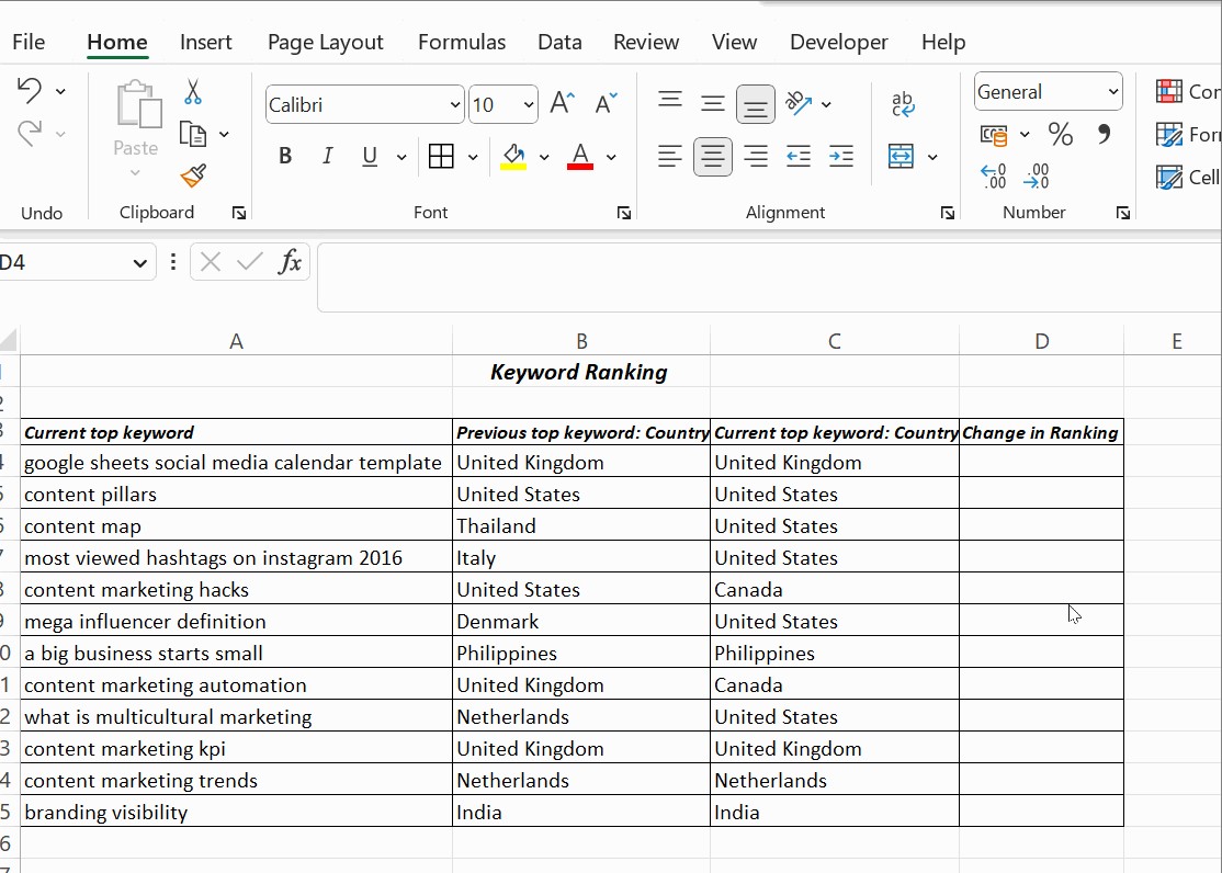
3. How To Use the Equals Operator to Compare Contents in Excel?
The equals operator (=) is a simple way to compare two columns row by row. It returns TRUE if the values in the compared columns are the same and FALSE if they differ.
Here’s how to use the equals operator:
- Select the first cell where you want to display the comparison result (e.g., D4).
- Enter the formula
=B4=C4and press Enter. - Drag the fill handle (the small square at the bottom right of the cell) down to apply the formula to the rest of the rows.
Excel will display TRUE for matching rows and FALSE for mismatched rows.
4. How To Compare Contents in Excel Using the IF Condition?
The IF condition allows you to return custom messages based on the comparison result. For example, you can display “Match” if the values are the same and “Not Match” if they are different.
Here’s how to use the IF condition:
- Select the first cell where you want to display the comparison result (e.g., D4).
- Enter the formula
=IF(B4=C4,"Match","Not Match")and press Enter. - Drag the fill handle down to apply the formula to the rest of the rows.
Excel will display “Match” for matching rows and “Not Match” for mismatched rows.
You can also use the IF condition to find differences between two columns by replacing the equals sign (=) with the not-equal-to sign (<>). The formula would be =IF(B4<>C4,"Different","Same").
5. What Is the EXACT Function and How to Use It for Case-Sensitive Comparisons in Excel?
The EXACT function compares two text strings and returns TRUE only if they are exactly the same, including case. This is useful when you need to ensure that the capitalization of the text is identical.
The syntax for the EXACT function is =EXACT(text1, text2).
Here’s how to use the EXACT function with the IF condition for case-sensitive comparisons:
- Select the first cell where you want to display the comparison result (e.g., D4).
- Enter the formula
=IF(EXACT(B4,C4), "Match", "Not Match")and press Enter. - Drag the fill handle down to apply the formula to the rest of the rows.
Excel will display “Match” only for rows where the text is exactly the same, including case.
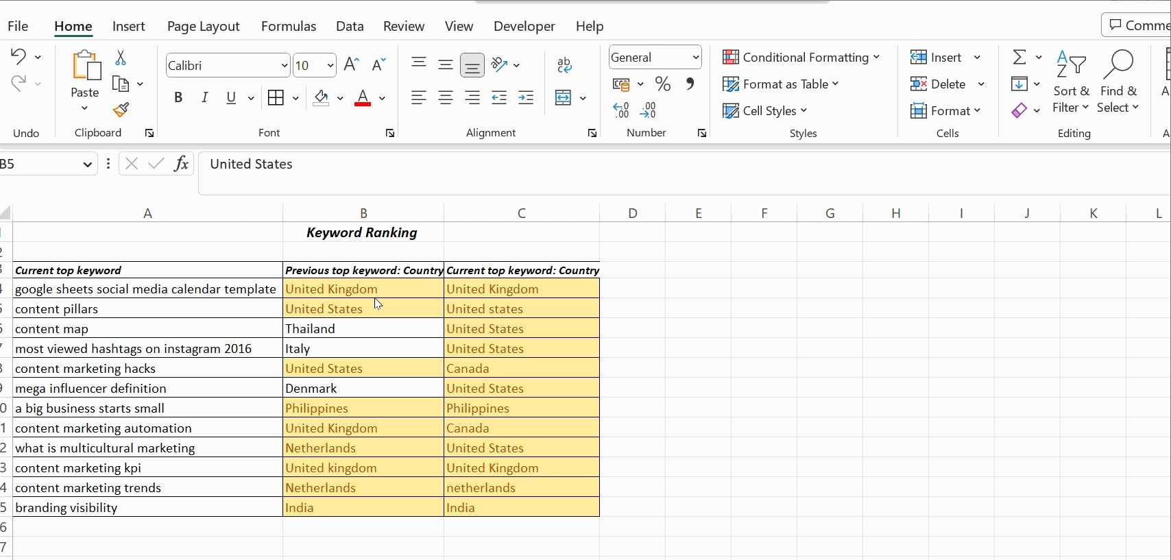
6. How To Use Conditional Formatting to Compare Contents in Excel?
Conditional formatting allows you to highlight cells based on certain criteria. You can use it to highlight duplicate or unique values in two columns, making it easy to identify matching or mismatched data.
Here’s how to use conditional formatting:
- Select the two columns you want to compare.
- Click Home > Conditional Formatting > Highlight Cells Rules > Duplicate Values.
- In the Duplicate Values dialog box, choose either Duplicate or Unique from the drop-down menu.
- Select a formatting style (e.g., light red fill with dark red text) or choose Custom Format to create your own style.
- Click OK.
Excel will highlight the duplicate or unique values in the selected columns based on your chosen criteria.
You can also clear the conditional formatting rules by clicking Conditional Formatting > Clear Rules > Clear Rules from Selected Cells.
7. How Do Lookup Functions Like VLOOKUP Help in Comparing Data in Excel?
Lookup functions, such as VLOOKUP, HLOOKUP, and XLOOKUP, are useful for finding matching values in different columns or tables. VLOOKUP (Vertical Lookup) searches for a value in the first column of a range and returns a corresponding value from another column in the same row.
Here’s an example of how to use VLOOKUP to compare two columns:
Suppose you have a list of product IDs in column A and a list of order IDs in column B. You want to find the corresponding order ID for each product ID.
- Select the cell where you want to display the result (e.g., C2).
- Enter the formula
=VLOOKUP(A2, B:B, 1, FALSE)and press Enter. - Drag the fill handle down to apply the formula to the rest of the rows.
The VLOOKUP function will search for the product ID in column A within column B and return the corresponding order ID. If the product ID is not found, it will return #N/A.
Understanding the VLOOKUP Formula:
A2: The lookup value (the value you want to find).B:B: The table array (the range where you want to search for the lookup value).1: The column index number (the column from which you want to return the matching value). In this case, it’s 1 because we’re searching in column B and want to return the value from the same column.FALSE: The range lookup (specifies whether you want an exact match or an approximate match). FALSE indicates that you want an exact match.
8. How Can I Compare Two Columns in Excel for Differences Using a Formula?
To compare two columns in Excel and highlight the differences, you can use a combination of the IF and ISNA functions along with the MATCH function. This method is particularly useful when you want to identify values in one column that are not present in another.
Here’s how you can do it:
-
Set Up Your Data:
- Assume you have two columns, A and B, with lists of data you want to compare.
- You want to find out which items in column A are not in column B.
-
Enter the Formula:
- In cell C1 (or any other column you prefer), enter the following formula:
=IF(ISNA(MATCH(A1,B:B,0)), "Not in B", "") - This formula checks if the value in cell A1 exists in column B. If it does not exist, it returns “Not in B”. If it exists, it returns an empty string.
- In cell C1 (or any other column you prefer), enter the following formula:
-
Drag the Formula Down:
- Click and drag the bottom-right corner of cell C1 down to apply the formula to all the rows you want to compare.
-
Explanation of the Formula:
MATCH(A1,B:B,0): This part of the formula searches for the value in cell A1 within the entire column B. The0specifies that you are looking for an exact match. If the value is found, MATCH returns the row number where the value is located. If the value is not found, MATCH returns#N/A.ISNA(MATCH(A1,B:B,0)): This checks if the result of the MATCH function is#N/A.ISNAreturnsTRUEif the value is#N/A(meaning the value in A1 is not found in column B) andFALSEotherwise.IF(ISNA(MATCH(A1,B:B,0)), "Not in B", ""): This is the main part of the formula. It checks the result of theISNAfunction. If it’sTRUE(i.e., the value in A1 is not found in column B), it returns the text “Not in B”. If it’sFALSE(i.e., the value is found in column B), it returns an empty string, making the cell appear blank.
Example
| A (List 1) | B (List 2) | C (Result) | |
|---|---|---|---|
| 1 | Apple | Banana | Not in B |
| 2 | Banana | Apple | |
| 3 | Cherry | Orange | Not in B |
| 4 | Date | Grape | Not in B |
| 5 | Elderberry | Cherry | Not in B |

In this example:
- Column A contains the first list of fruits.
- Column B contains the second list of fruits.
- Column C uses the formula
=IF(ISNA(MATCH(A1,B:B,0)), "Not in B", "")to check if each fruit in column A is present in column B. - The result in column C indicates which fruits from column A are not found in column B.
Additional Tips
- Adjusting the Columns: Make sure to adjust the column references in the formula according to your actual data.
- Handling Large Datasets: For very large datasets, consider using array formulas or more advanced techniques to improve performance.
- Using Conditional Formatting: You can combine this formula with conditional formatting to highlight the “Not in B” cells for better visual identification.
This method provides a clear and efficient way to compare two columns in Excel for differences, allowing you to quickly identify and address any discrepancies in your data.
9. How to Compare Two Columns in Excel and Return Value from Third Column?
Comparing two columns in Excel and returning a value from a third column based on that comparison can be achieved using a combination of the IF and VLOOKUP (or INDEX and MATCH) functions. Here’s how you can do it:
Method 1: Using IF and VLOOKUP
-
Set Up Your Data:
- Assume you have three columns: A, B, and C.
- Columns A and B contain the data you want to compare.
- Column C contains the values you want to return based on the comparison.
-
Enter the Formula:
-
In cell D1 (or any other column you prefer), enter the following formula:
=IF(A1=B1, VLOOKUP(A1, A:C, 3, FALSE), "No Match")
-
-
Drag the Formula Down:
- Click and drag the bottom-right corner of cell D1 down to apply the formula to all the rows you want to compare.
-
Explanation of the Formula:
-
IF(A1=B1, ..., "No Match"): This part of the formula compares the values in cells A1 and B1. If they are equal, it proceeds to execute theVLOOKUPfunction. If they are not equal, it returns “No Match”. -
VLOOKUP(A1, A:C, 3, FALSE): If the values in A1 and B1 are equal, this function searches for the value of A1 in column A, looks through columns A to C, and returns the value from the third column (Column C).A1: The lookup value (the value you want to find).A:C: The table array (the range where you want to search for the lookup value and return a corresponding value).3: The column index number (the column from which you want to return the matching value). In this case, it’s 3 because you want to return the value from Column C.FALSE: The range lookup (specifies that you want an exact match).
-
Method 2: Using IF and INDEX/MATCH
The INDEX and MATCH functions can be more flexible and efficient than VLOOKUP, especially when dealing with large datasets.
-
Set Up Your Data:
- Same as Method 1: three columns (A, B, and C) with data to compare and a column with values to return.
-
Enter the Formula:
-
In cell D1, enter the following formula:
=IF(A1=B1, INDEX(C:C, MATCH(A1, A:A, 0)), "No Match")
-
-
Drag the Formula Down:
- Click and drag the bottom-right corner of cell D1 down to apply the formula to all the rows.
-
Explanation of the Formula:
-
IF(A1=B1, ..., "No Match"): Same as Method 1, it compares the values in cells A1 and B1. -
INDEX(C:C, MATCH(A1, A:A, 0)): If the values in A1 and B1 are equal, this function usesINDEXandMATCHto find the corresponding value in Column C.-
MATCH(A1, A:A, 0): This finds the row number where the value in A1 is located in Column A.A1: The lookup value.A:A: The lookup array (Column A).0: Specifies an exact match.
-
INDEX(C:C, ...): This returns the value from Column C at the row number found by theMATCHfunction.
-
-
Example
| A (Data 1) | B (Data 2) | C (Return Value) | D (Result) | |
|---|---|---|---|---|
| 1 | 101 | 101 | Apple | Apple |
| 2 | 102 | 103 | Banana | No Match |
| 3 | 103 | 103 | Cherry | Cherry |
| 4 | 104 | 105 | Date | No Match |
| 5 | 105 | 105 | Elderberry | Elderberry |
In this example:
- Columns A and B are compared.
- If the values in Columns A and B are equal, the corresponding value from Column C is returned in Column D.
- If the values in Columns A and B are not equal, “No Match” is returned in Column D.
Additional Tips
-
Adjusting the Columns:
- Make sure to adjust the column references in the formula according to your actual data.
-
Handling Errors:
-
If the
VLOOKUPorINDEX/MATCHfunctions do not find a match, they will return an error (#N/A). You can handle these errors using theIFERRORfunction:=IFERROR(IF(A1=B1, VLOOKUP(A1, A:C, 3, FALSE), "No Match"), "Not Found")or
=IFERROR(IF(A1=B1, INDEX(C:C, MATCH(A1, A:A, 0)), "No Match"), "Not Found")This will return “Not Found” if there is an error.
-
By using these methods, you can effectively compare two columns in Excel and return a value from a third column based on whether the values in the first two columns match. This is particularly useful for data validation, data enrichment, and creating dynamic reports.
10. How To Compare Multiple Columns in Excel?
Comparing multiple columns in Excel requires a slightly more complex formula. You can use the IF and AND functions to check if all the values in the columns are the same.
Here’s how to compare three or more columns:
- Select the cell where you want to display the comparison result (e.g., E2).
- Enter the formula
=IF(AND(A2=B2, A2=C2, B2=C2), "Match", "Not Match")and press Enter. - Drag the fill handle down to apply the formula to the rest of the rows.
This formula checks if the values in columns A, B, and C are the same. If they are, it returns “Match”. Otherwise, it returns “Not Match”.
You can also modify the formula to find matches in any two cells in the same row:
=IF(OR(A2=B2, B2=C2, A2=C2), "Match", "Not Match")
This formula returns “Match” if any two cells in the row have the same value.
11. What Are Some Advanced Techniques for Comparing Contents in Excel?
For more complex comparisons, you can use advanced techniques such as:
- Array Formulas: Perform calculations on multiple values at once.
- Macros (VBA): Automate repetitive tasks and create custom comparison functions.
- Power Query: Import and transform data from multiple sources for comparison.
These techniques require more advanced Excel skills, but they can be very powerful for handling large and complex datasets.
12. How to Compare Two Lists in Excel and Find Matches?
To compare two lists in Excel and find matches, you can use a combination of the COUNTIF function and conditional formatting. This method will highlight the values that appear in both lists.
Steps
-
Set Up Your Data:
- Assume you have two lists in columns A and B.
- You want to find the values that are present in both lists.
-
Use
COUNTIFto Identify Matches:-
In cell C1, enter the following formula:
=COUNTIF(B:B, A1) -
Drag the formula down to apply it to all the rows in column A.
-
-
Explanation of the Formula:
-
COUNTIF(B:B, A1): This function counts how many times the value in cell A1 appears in column B.B:B: The range to search (i.e., column B).A1: The criteria (i.e., the value to count).
-
If the result is greater than 0, it means the value in A1 is present in column B.
-
-
Apply Conditional Formatting to Highlight Matches:
-
Select the range of cells in column A where you want to highlight the matches (e.g., A1:A10).
-
Go to Home > Conditional Formatting > New Rule.
-
Select “Use a formula to determine which cells to format”.
-
Enter the following formula in the formula box:
=COUNTIF(B:B, A1)>0 -
Click the Format button to choose the formatting style you want to apply (e.g., fill color, font color).
-
Click OK to close the format window, and then click OK again to create the rule.
-
Example
| A (List 1) | B (List 2) | C (Count) | |
|---|---|---|---|
| 1 | Apple | Banana | 0 |
| 2 | Banana | Apple | 1 |
| 3 | Cherry | Orange | 0 |
| 4 | Date | Grape | 0 |
| 5 | Elderberry | Cherry | 1 |
In this example:
- Column A contains the first list of fruits.
- Column B contains the second list of fruits.
- Column C uses the formula
=COUNTIF(B:B, A1)to count how many times each fruit in column A appears in column B. - The conditional formatting highlights the fruits in column A that are also found in column B.
Additional Tips
-
Adjusting the Columns:
- Make sure to adjust the column references in the formula according to your actual data.
-
Using a Helper Column:
-
Instead of using conditional formatting, you can use the
IFfunction to display a message if there’s a match:=IF(COUNTIF(B:B, A1)>0, "Match", "")This formula will display “Match” in column C if the value in column A is found in column B.
-
-
Comparing Two Columns for Differences:
-
To find values that are in one list but not the other, you can use the
IFandISNAfunctions withMATCH:=IF(ISNA(MATCH(A1, B:B, 0)), "Not in B", "")
-
By using these methods, you can efficiently compare two lists in Excel and find matches, allowing you to quickly identify common values and discrepancies. This is particularly useful for data validation, data cleaning, and creating reports.
13. How To Compare Two Excel Sheets for Differences?
Comparing two Excel sheets for differences can be achieved using several methods, depending on the complexity and structure of your data. Here are a few common techniques:
Method 1: Using Conditional Formatting
This method is useful for visually highlighting differences between two sheets, assuming the data is in the same format and order.
-
Open Both Excel Sheets:
- Make sure both Excel sheets you want to compare are open.
-
Select the Data Range in the First Sheet:
- Select the range of cells in the first sheet that you want to compare (e.g., A1:C10).
-
Apply Conditional Formatting:
-
Go to Home > Conditional Formatting > New Rule.
-
Select “Use a formula to determine which cells to format”.
-
Enter the following formula (adjust the sheet name and cell references as needed):
=A1<>Sheet2!A1 -
Click the Format button to choose the formatting style you want to apply (e.g., fill color, font color).
-
Click OK to close the format window, and then click OK again to create the rule.
-
-
Explanation of the Formula:
A1<>Sheet2!A1: This formula compares the value in cell A1 of the first sheet with the value in cell A1 of the second sheet. If they are different, the formula returnsTRUE, and the conditional formatting is applied.
Method 2: Using a Formula to Check for Differences
This method allows you to create a new column that indicates whether each row is the same or different between the two sheets.
-
Open Both Excel Sheets:
- Make sure both Excel sheets you want to compare are open.
-
Insert a New Column in the First Sheet:
- Insert a new column next to the data you want to compare (e.g., column D).
-
Enter the Formula:
-
In cell D1, enter the following formula (adjust the sheet name and cell references as needed):
=IF(A1=Sheet2!A1, "Same", "Different")
-
-
Drag the Formula Down:
- Click and drag the bottom-right corner of cell D1 down to apply the formula to all the rows you want to compare.
-
Explanation of the Formula:
IF(A1=Sheet2!A1, "Same", "Different"): This formula compares the value in cell A1 of the first sheet with the value in cell A1 of the second sheet. If they are the same, it returns “Same”. If they are different, it returns “Different”.
Method 3: Using Power Query (Get & Transform Data)
This method is more robust for comparing sheets with different structures or when you need to identify added or removed rows.
-
Open a New Excel Workbook:
- Open a new Excel workbook to perform the comparison.
-
Import Data from Both Sheets:
- Go to Data > Get & Transform Data > From Table/Range.
- Select the range of data in the first sheet and click OK. This will open the Power Query Editor.
- Rename the query (e.g., “Sheet1”).
- Close & Load To… > Only Create Connection.
- Repeat the process for the second sheet (e.g., rename the query to “Sheet2”).
-
Create a Merged Query:
- Go to Data > Get & Transform Data > Get Data > Combine Queries > Merge.
- In the Merge dialog box:
- Select “Sheet1” as the first table.
- Select “Sheet2” as the second table.
- Select the columns you want to use for matching (e.g., ID, Name).
- Choose the join kind (e.g., “Left Outer” to keep all rows from Sheet1 and matching rows from Sheet2).
- Click OK.
-
Expand the Merged Column:
- Click the expand button (two arrows pointing outwards) in the header of the merged column (e.g., “Sheet2”).
- Select the columns you want to expand from Sheet2 and click OK.
-
Add a Custom Column to Check for Differences:
-
Go to Add Column > Custom Column.
-
Enter a formula to check for differences (e.g., if you have columns “Value1” from Sheet1 and “Value2” from Sheet2):
= if [Value1] = [Value2] then "Same" else "Different" -
Click OK.
-
-
Load the Results:
- Go to Home > Close & Load To… > Table > New Worksheet.
- Click Load.
Example
Sheet1
| ID | Name | Value1 | |
|---|---|---|---|
| 1 | 1 | Apple | 10 |
| 2 | 2 | Banana | 20 |
| 3 | 3 | Cherry | 30 |
| 4 | 4 | Date | 40 |
Sheet2
| ID | Name | Value2 | |
|---|---|---|---|
| 1 | 1 | Apple | 10 |
| 2 | 2 | Banana | 25 |
| 3 | 3 | Cherry | 30 |
| 4 | 5 | Elderberry | 50 |
Merged Query Result (using Power Query)
| ID | Name | Value1 | Value2 | Status | |
|---|---|---|---|---|---|
| 1 | 1 | Apple | 10 | 10 | Same |
| 2 | 2 | Banana | 20 | 25 | Different |
| 3 | 3 | Cherry | 30 | 30 | Same |
| 4 | 4 | Date | 40 | null | Different |
| 5 | 5 | Elderberry | null | 50 | Different |
Additional Tips
- Handling Different Structures:
- Power Query is particularly useful when the sheets have different column orders or structures. You can use transformations within Power Query to align the data before comparing.
- Error Handling:
- Use
IFERRORin your formulas to handle errors that may occur if data is missing or inconsistent.
- Use
- Large Datasets:
- For very large datasets, Power Query is generally more efficient than using formulas directly in Excel.
By using these methods, you can effectively compare two Excel sheets for differences, identify discrepancies, and ensure data accuracy. Choose the method that best suits the complexity and structure of your data.
14. What Are Some Common Mistakes to Avoid When Comparing Contents in Excel?
When comparing contents in Excel, it’s important to avoid common mistakes that can lead to inaccurate results. These mistakes include:
- Ignoring Case Sensitivity: Use the EXACT function when case matters.
- Not Locking Cell References: Use absolute references ($) when comparing against a fixed range.
- Assuming Data Consistency: Check for leading or trailing spaces, different data types, and formatting inconsistencies.
- Overlooking Hidden Rows or Columns: Make sure all data is visible and included in the comparison.
- Not Testing Formulas: Always test your formulas with sample data to ensure they produce the correct results.
By avoiding these mistakes, you can ensure that your comparisons are accurate and reliable.
15. How Can COMPARE.EDU.VN Help Me Compare Contents in Excel More Effectively?
COMPARE.EDU.VN offers a variety of resources to help you compare contents in Excel more effectively. Our website provides:
- Detailed Tutorials: Step-by-step instructions on how to use different Excel comparison techniques.
- Template Files: Pre-built Excel templates with formulas and conditional formatting set up for common comparison scenarios.
- Expert Advice: Tips and tricks from Excel experts on how to optimize your comparisons and avoid common mistakes.
- Community Forum: A place to ask questions and get help from other Excel users.
By using COMPARE.EDU.VN, you can save time, improve accuracy, and gain valuable insights from your data.
Conclusion
Comparing contents in Excel is a crucial skill for data analysis and decision-making. By using the techniques outlined in this guide, you can efficiently compare data across columns and spreadsheets, identify discrepancies, and ensure data consistency. Remember to choose the right method for your specific needs and avoid common mistakes to ensure accurate results.
Ready to take your Excel skills to the next level? Visit COMPARE.EDU.VN today to access detailed tutorials, template files, and expert advice on comparing contents in Excel. Our resources will help you save time, improve accuracy, and gain valuable insights from your data.
Address: 333 Comparison Plaza, Choice City, CA 90210, United States
WhatsApp: +1 (626) 555-9090
Website: compare.edu.vn
Frequently Asked Questions (FAQs)
1. How do I compare two columns in Excel for exact matches?
To compare two columns for exact matches, use the EXACT function within an IF statement. For example, =IF(EXACT(A1, B1), "Match", "No Match"). This formula checks if the content of cell A1 is exactly the same as the content of cell B1, including case sensitivity.
2. Can I compare data in Excel without using formulas?
Yes, you can use conditional formatting to highlight differences or duplicates without using formulas. Select the columns, go to Home > Conditional Formatting > Highlight Cells Rules, and choose Duplicate Values or use a formula-based rule to highlight differences.
3. How do I compare two Excel files for differences?
You can compare two Excel files by opening both and using a formula like =IF(Sheet1!A1=Sheet2!A1, "Same", "Different") to compare cell values. Alternatively, use Power Query to import data from both files and merge them based on common columns to identify discrepancies.
4. What is the best way to compare large datasets in Excel?
For large datasets, using Power Query is often the most efficient method. It allows you to import, transform, and compare data from multiple sources, identify differences, and load the results into a new sheet.
5. How do I find unique values in two columns in Excel?
To find unique values, use conditional formatting or the COUNTIF function. For conditional formatting, select the data and create a new rule using the formula =COUNTIF($A:$B, A1)=1 to highlight unique values.
6. How can I compare two columns and return a value from another column if there is a match?
Use the VLOOKUP function. For example, if you want to compare column A to column B and return a value from column C when there’s a match, use the formula =IF(ISNA(VLOOKUP(A1, B:C, 2, FALSE)), "No Match", VLOOKUP(A1, B:C, 2, FALSE)).
7. Is there a way to automate the comparison of Excel sheets?
Yes, you can automate the comparison of Excel sheets using VBA (Visual Basic for Applications) macros. You can write a macro to loop through the cells in both sheets and highlight or flag differences.
8. How do I ignore case sensitivity when comparing two columns in Excel?
To ignore case sensitivity, use the UPPER or LOWER functions to convert both columns to the same case before